B M B 400

Part Four: Gene Regulation

Section II = Chapter 17.

TRANSCRIPTIONAL REGULATION EXERTED BY EFFECTS ON RNA POLYMERASE

[Dr. Tracy Nixon made major contributions to this chapter.]

A. The multiple steps in initiation and elongation by RNA polymerase are targets for regulation.

1. RNA Polymerase has to

* bind to promoters,

* form an open complex,

* initiate transcription,

* escape from the promoter,

* elongate , and

* terminate transcription.

See Fig. 4.2.1.

2. Summarizing a lot of work, we know that:

• strong promoters have high KB, high kf, low kr, and high rates of promoter clearance.

• weak promoters have low KB, low kf, high kr, and low rates of promoter clearance.

• moderate promoters have one or more "weak" spots.

3. To learn these facts, we need:

• genetic data to identify which macromolecules (DNA and proteins) interact in a specific regulation event, and to determine which base pairs and amino acid residues are needed for that regulation event.

• biochemical data to describe the binding events and chemical reactions that are affected by the specific regulation event. Ideally, we would determine all forward and reverse rate constants, or equilibrium constants (which are a function of the ratio of rate constants) if rates are inaccessible. Although, in reality, we cannot get either rates or equilibrium constants for many of the steps, some of the steps are amenable to investigation and have proved to be quite informative about the mechanisms of regulation.

Fig. 4.2.1

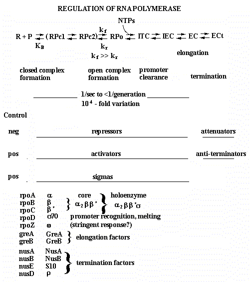
Pc = closed promoter complex, Po = open promoter complex, ITC = initial transcribing complex, IEC = initial elongating complex, EC = elongation complex, ECt = terminating elongation complex.

B. Methods exist for measuring rate constants and equilibrium constants, and newer, more accurate methods are now being used.

1. Classical methods of equilibrium studies and data analysis

o use low concentrations of enzymes and make assumptions that

simplify complex reactions so that they can be treated by definite

integrals of chemical flux equations

o manipulate an equation into a form that can be plotted as a linear

function, and derive parameter estimates by slope and intercept

values

2. Driven by the success of recombinant DNA and protein purification

technology, and by the increased computational power in desktop

computers, the classical methods are being replaced by

o using of large amounts of enzymes to directly include them in

kinetic studies. In this approach, the enzymes are used in substrate level quantities.

o numerical integrations of chemical flux equations (Kinetic Simulation)

o more rigorous methods based on NonLinear, Least Squares (NLLS)

regression, and

o analyzing data from multiple experiments of different design

simultaneously (global NLLS analysis).

3. These changes

* increase the steps in a reaction that can be examined experimentally

* replace the limited set of simple mechanisms that can be analyzed with

essentially any mechanism

* increase knowledge of error, permitting conclusions to be drawn with

more confidence

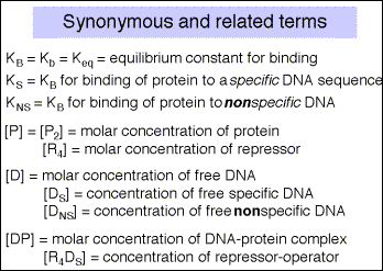
Box 1: The equations used in this chapter come from several different sources that use different names for the same thing. The following lists some of these synonyms.

C. Experimental approaches to macromolecular binding reactions

Several methods are available for measuring the amount of protein that binds specifically to a DNA molecule. We have already encountered these as methods for localizing protein-binding sites on DNA, and all are amenable to quantitation.

Major methods include nitrocellulose filter binding, electrophoretic mobility shift assays, and DNase protection assays.

Which Experimental Technique is Best?

* The kind of observations that can be made about the system differ for

different experimental approaches.

* These differences lead to specific problems with each technique,

* Each technique depends on combining the analysis of more than one

experiment to obtain enough information to resolve intrinsic binding

free energy from cooperativity energy.

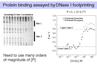
Fig. 4.2.2

Data courtesy of Dr. Tracy Nixon

The most robust technique is DNase I footprinting. If you are studying the binding of multiple, interacting proteins, then it is possible that these proteins are showing cooperativity in their binding to DNA. When analyzing such cooperativity by DNase I footprinting, the resolution is limited to cooperativities >0.5 kcal/mole, and is subject to some critical assumptions. Gel-shifts (also called electrophoretic mobility shift assays, or EMSAs) are useful when there is no cooperativity, or when cooperativity is large relative to site heterogeneity. Filter binding studies require knowledge about filter retention efficiencies for the different protein-DNA complexes, which can only be empirically determined. And always keep in mind that flanking sequences do affect binding affinities, and even point mutations can have distant effects.

In any of these assays, we are devising a physical means for measuring a quantity that is related to fractional occupancy.

D. Measurement of equilibrium constants in macromolecular binding reactions

1. Classical methods with their linear transformation are not as accurate as the NonLinear, Least Squares (NLLS) regression analysis, but they can serve to show the general approach.

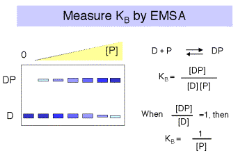
a. The binding constants can be determined by titrating labeled DNA binding sites with increasing amounts of the repressor, and measuring amount of protein-bound DNA and the amount of free DNA. Typical techniques are electrophoretic mobility shift assays or nitrocellulose filter binding.

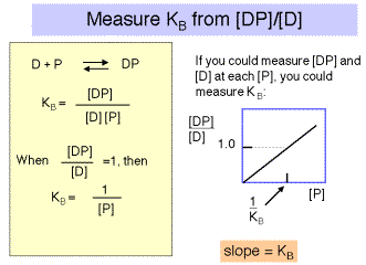
Note that for a simple equilibrium of a single protein binding to a single site on the DNA, the equilibrium constant for binding (K_B) is approximated by the inverse of the protein concentration at which the concentration of DNA bound to protein equals the concentration of free DNA (Fig. 4.2.3).

Fig. 4.2.3

If it were possible to reliably determine both the concentration of DNA bound to protein (i.e. [DP]) and the concentration of free DNA ([D]), then one could plot the ratio of bound DNA to free DNA at each concentration of repressor. If the results were linear, then the slope of the line would give the equilibrium binding constant, KB . See Fig. 4.2.4.

Fig. 4.2.4

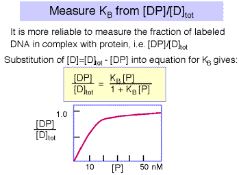
However, the error associated with determining very low concentrations of free or bound DNA is substantial, and a more reliable measurement is that of the ratio of bound DNA to total DNA, i.e. [DP]/[D]_tot , as illustrated in Fig. 4.2.5. The equation describing this binding curve has a form equivalent to the Michelis-Menten equation for steady-state enyzme kinetics. Note that the concentration of protein at which half the DNA is bound to protein is the inverse of K_B . You can show this for yourself by substituting 0.5 for [DP]/[D]_tot in the equation. At this point, [P] = 1/K_B .

Fig. 4.2.5.

2. Problems with the classical approach.

In this classical approach, experiments were designed such that

o one or more concentrations could be assumed to be unchanging, and

o observations were manipulated mathematically (transformed) to a linear equation so that one could

+ plot the transformed data,

+ decide where to draw a straight line, and

+ use the slope and intercepts to estimate the parameters in question.

(Scatchard plots, Lineweaver-Burke plots, etc).

* Two problems are associated with the older technique

o Deciding where to draw the straight line is an arbitrary decision

for each person doing the analysis (and using a linear regression

to find the "best fit" line is not justified, as two of the

assumptions about your data that are needed to justify such a

regression are not true)

o There is no accurate estimate of the error in the estimate of the

parameter value

3. These limitations have been overcome in the last 5 or so years, aided by the advent of recombinant DNA techniques that allow the production of large amounts of the proteins being analyzed, and the availability of powerful microcomputers that can carry out the large number of computations required for nonlinear, least squares regression analysis (NLLS).

a. We can model binding reactions by

• tabulating the different states that exist in a system,

• associating each state with a fractional probability based on the Boltzmann partition function and the Gibb's free energy for that state (DGs),

• and determine the probability of any observed measurement by the ratio of

o the sum of fractional probabilities that give the observation, and

o the sum of the fractional probabilities of all possible states.

Where j is the number of ligands bound, the fractional probability of a particular state is given by this equation for fs .

As an example, consider a one-site system, such as an operator that binds one protein. There are two states, the 0 state with no protein bound to the operator and the 1 state with one protein bound. Thus one can write the equation for f0 and for f1 .

If we expand the fractional probabilities for each of these fractional occupancy equations, we derive equations relating fractional occupancy, , to a function of Gibb's free energies for binding (DG), protein concentration ([P2]), and complex stoichiometry (j).

For a single site system, we have the following equations:

Since Gibb's free energy is also related to the equilibrium constant for reactions:

DG = -RT ln (Keq)

these free energies can be re-cast as equilibrium constants, as follows.

A more complete presentation of this method, including a treatment of multiple binding sites, can be obtained at the BMB Courses web site (http://www.bmb.psu.edu/courses/default.htm) by clicking on BMB400 "Nixon Lectures."

b. Analyzing the data

After collecting the binding data, we are in a position to analyze the observed data to find out what values for DG or Kb make the function best predict the observations. Statisticians have developed Maximum Likelihood Theory to allow using the data to find, for each parameter, the value that is most likely to be correct. For biochemical data the approach that is most appropriate (most of the time) is global, nonlinear, least squares (NLLS) regression.

• Fortunately, desktop computers are now powerful enough to do these calculations in a few minutes, for one experiment, or even for many experiments combined in a global analysis. This method has several advantages. It gives you:

o the same parameter estimates, no matter what program or method you or someone else uses, provided that the program is written correctly and used correctly.

o much more rigorous estimates of error.

This last point is worth emphasizing:

• is it not true that $100 (minus $50) is much less attractive

as a fee for your time than is $100 (minus $0.01)? The same

can be true for estimates of binding free energies, or

equilibrium constants .

• Moreover, when several experiments are required to estimate a

parameter, the error in each experiment should be included in

the estimate of the parameter. Without a global analysis that

determines a conglomerate error, it is not possible to

carefully carry forward the error of one experiment to the

analysis of data from additional ones.

c. This analysis produces a plot of the variance of fit, or error, over a wide range of possible values for the parameter being measured, such as the DG for binding. The DG value with the smallest error is the most accurate value.

An example of this analysis is shown in Fig. 4.2.6. The raw data shown in Fig. 4.2.2 (left panel) produced the binding curves shown on right panel of that figure. These data were then subjected to non-linear least-squares analysis. The errors (or variance of fit) for each possible value of DG are plotted in Fig. 4.2.6. For example, note that the lowest variance of fit for DG₁ is about –9.5 kcal/mole.

Fig. 4.2.6.

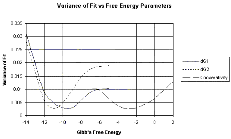
dG1 = DG1 = Gibb's free energy for binding to the first site of a two-site system.

dG2 = DG2 = Gibb's free energy for binding to the second site of a two-site system.

The variance of fit for the DG for the cooperativity between proteins bound at the two sites is also plotted.

These data were kindly provided by Dr. Tracy Nixon.

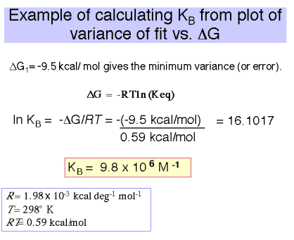
As indicated above, once a value for DG is available, one can calculate Keq from

DG = -RT ln (Keq)

Fig. 4.2.7.

Some key references for NLLS:

Senear and Bolen, 1992, Methods Enzymol. 210:463

Koblan et al, 1992, Methods Enzymol. 210:405.

Senear et al 1991, J. Biol. Chem. 266:13661

E. Insights into the mechanism of lac regulation by measuring binding constants.

1. Having gone through both classical and non-linear least squares analysis for measuring binding constants, let’s look at an example of how one uses these measurements to better understand the mechanism of gene regulation. We know that transcription of the lac operon is increased in the presence of the inducer, but how does this occur? One could list a number of possibilities, each with different predictions about how the inducer may affect the binding constant of repressor for operator, K_B.

a. Does the inducer change the conformation of the lac repressor so that it now activates transcription? This could occur with no effect on K_B.

b. Does inducer cause the repressor to dissociate from the operator DNA and remain free in solution? This predicts a decrease in K_B for specific DNA, but no binding to nonspecific DNA.

c. Does inducer cause the repressor to dissociate from the operator and redistribute to nonspecific sites on the DNA? This predicts a decrease in K_B for specific DNA, but proposes that most of the repressor is bound to non-operator sites.

Measurement of the equilibrium constants for lac repressor binding to operator and to nonspecific DNA, in the absence and presence of the inducer, shows that possibility c above is correct. This section of the chapter explores this result in detail.

2. In the absence of inducer, the repressor, or R₄, will bind to specific sites (in this case the operator) with high affinity and to nonspecific sites (other DNA sequences) with lower affinity (Fig. 4.2.8). This is stated quantitatively in the following values for the equilibrium association constant. Either equilibrium constant can be abbreviated Keq or KB. We will use the term KS to refer to KB at specific sites and KNS for the KB at nonspecific sites.

KS = 2 x 1013 M-1 KNS = 2 x 106 M-1

[A detailed presentation of some representative data and how to use them to determine these binding constants for the lac repressor is in Appendix A at the end of this chapter. This Appendix goes through the classic approach to measuring binding constants.]

3. The binding constant of lac repressor to its operator changes in the presence of inducer. (Fig. 4.2.8)

Binding of the inducer to the repressor lowers the affinity of the repressor for the operator 1000 fold, but does not affect the affinity of repressor for nonspecific sites.

For R4 with inducer :

KS = 2 x 1010 M -1 KNS = 2 x 106 M -1

Fig. 4.2.8.

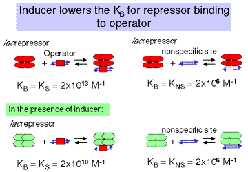
4. The difference in affinity for specific versus nonspecific sites can be described by the specificity parameter, which is the ratio between the equilibrium constant for specific binding and the equilibrium constant for nonspecific binding.

Specificity = in absence of inducer

in presence of inducer

Note the in the presence of the inducer, the specificity with which the lac repressor binds to DNA is decreased 1000-fold.

Even though the repressor still has a higher affinity for specific DNA in the presence of the inducer, there are so many nonspecific sites in the genome that the repressor stays bound to these nonspecific sites rather than finding the operator. Hence in the presence of the inducer, the operator is largely unoccupied by repressor, and the operon is actively transcribed.

The regulation of the lac operon via redistribution of the repressor to nonspecific sites in the genome is covered in more detail in the next two sections. They show the effect of having a large number of nonspecific, low affinity sites competing with a single, high affinity site for a small number of repressor molecules.

5. Distribution of repressor between operator and nonspecific sites

Although repressor has a much higher affinity for the operator than for nonspecific sites, there are so many more nonspecific sites (4.6 x 106, since essentially every nucleotide in the E. coli genome is the beginning of a nonspecific binding site) than specific sites (one operator per genome) that virtually all of the repressor is bound to DNA, even if only nonspecific sites are present.

a. We use the binding constants above, and couple them with a calculation that the concentration of repressor (10 molecules per cell) is 1.7 x 10-8 M and the concentration of nonspecific sites (4.6 x 106 per cell) is 7.64 x 10-3 M. These values for [R4] and [DNS] are essentially constant. With this information, we can compute that the ratio of free repressor to that bound to nonspecific sites is less that 1 x 10-4 ( it is about 6.6 x 10-5), as shown in the box below. Thus only about 1 in 15,000 repressor molecules is not bound to DNA.

b. This analysis shows that the lac repressor is partitioned between nonspecific sites and the operator. When it is not bound to the operator, it is bound elsewhere to any of about 4.6 million sites in the genome. Almost none of the repressor is unbound to DNA in the cell.

c. Box 2 (below) goes through these calculations in more detail.

Box 2. Effectively all repressor protein is bound to DNA.

6. Regulation of the lac operon via redistribution of the repressor to nonspecific sites in the genome.

a. The high specificity of repressor for the operator means that in the absence of inducer, the operator is bound by the repressor virtually all the time. This is true despite the huge excess of nonspecific binding sites.

b. The specificity parameter described above (Ks/Kns) allows one to evaluate the simultaneous equilibria (repressor for operator and repressor for nonspecific sites on the DNA). We want to calculate the ratio of repressor-bound operators to free operators. Values for KS, KNS, and [DNS] are already known, and the concentration of repressor not bound to DNA is negligible.

Box 3. Specificity parameter is related to ratio of bound to free operator sites.

Specificity =

ratio of Bound:Free

operator sites

Now we need a value for [R4DNS]. This is obtained by realizing that under conditions that saturate specific sites, the concentration of repressor bound to nonspecific sites is closely approximated by [repressor]total - [operator], or [R₄]_total - [D_s]_total in the equations in Box 4.

Box 4.

[R4]free is negligible (see above).

Under conditions that saturate specific sites,

Thus [R4DNS] = [R₄]_total - [D_s]_total

c. After making these simplifying assumptions, we now have a value for every variable and constant in the equation, except the ratio of bound:free operator sites. Thus we can compute the desired ratio.

Box 5. Equation relating specificity to the ratio of bound to free operator and a set of constants.

Specificity =

already want to constants

measured determine

d. Now that we have the equation in Box 5, we can calculate the ratio of free operator to operator bound by repressor can be calculated in the absence and presence of inducer.

(1) In the absence of inducer:

Specificity =

i.e. the ratio of free operators to operators bound by repressor is 0.05. R4 is bound to the operator ~ 95% of the time. Thus the operon is not expressed.

(2) In the presence of inducer:

Specificity =

i.e. in the presence of inducer, only about 2% of the operators are bound by repressor, or R4 is bound to the operator ~ 2% of the time. Thus the operon is expressed.

In summary, these calculations show that in the absence of inducer, 95% of the operators are occupied (o is bound by R4 95% of the time). In the presence of inducer, the repressor re-distributes to nonspecific sites on the DNA, leaving only 2% of the operators bound by R4. Thus the operon is expressed in most of the cells.

An additional example of the use of the measured binding constants and the specificity parameter is in Appendix B at the end of this chapter. This example explores the effects of operator mutants.

F. Mechanism of repression and induction for the lac operon

1. Effect of lac repressor on the ability of RNA polymerase to bind to the promoter

The analysis in the previous section showed how the inducer affects the partitioning of the repressor between specific and nonspecific sites. Now let’s examine the effect that repressor bound to the operator has on the function of the polymerase at the promoter

Figure 4.1.9.

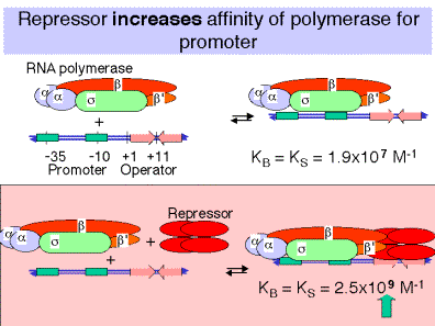
a. Binding of repressor to the operator actually increases the affinity of the RNA polymerase for the promoter!

Consider the following equilibrium:

RNA polymerase + promoter RNA polymerase-promoter (closed complex)

In the absence of repressor on the operator, the affinity of RNA polymerase for the lac promoter is

KB = 1.9 x 107 M-1

In the presence of repressor on the operator, the affinity is

KB = 2.5 x 109 M-1

b. Repressor bound to the operator increases the affinity of RNA polymerase for the lac promoter about 100 fold, so the closed complex is formed much more readily. The repressor essentially holds the RNA polymerase in storage at the promoter, but transcription is not initiated.

c. Upon binding of the inducer to the repressor, the repressor dissociates and the RNA polymerase-promoter complex can shift to the open complex and initiate transcription, thus switching on the operon.

d. Thus the effect of repressor bound to the operator is not on Kb for the polymerase-promoter interaction, but rather is on kf for the conversion from closed to open complex.

G. Kinetic measurements of the abortive initiation reaction allow one to calculate kf .

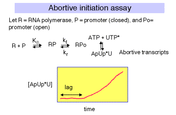
1. Abortive Transcription Assay

The initial transcribing complex (ITC) that exists after open complex formation frequently fails to transform into the initial elongating complex (IEC). The RNA product is released, and the system initiates again.

The rate at which the aborted transcripts accumulates can provide a measure of promoter strength, and experiments have been devised to use such an assay to estimate KB for polymerase binding to the promoter region, and kf for isomerization from closed to open complex form.

Polymerase, promoter DNA, and nucleotides are mixed such that a radiolabeled phosphate will be introduced into transcripts that are made and aborted. The amount of radioactivity in the short transcripts is then counted as a function of time.

Fig. 4.2.10

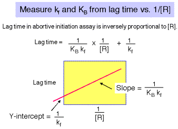
There is a lag between mixing reagents, and optimal rate of abortive transcript production. The length of this lag is inversely proportional to the [RNAP]. A plot of lag-time vs 1/[RNAP] gives a straight line plot, with slope equal to 1/[KB ´ kf] and y-intercept of 1/kf.

Fig. 4.2.11.

H. Activation of transcription by the CAP protein of E. coli

1. Activation of transcription by the CAP protein of E. coli illustrates several general regulatory principles.

We will focus on the point that in different contexts (different promoters), a single protein can directly interact with RNAP via at least 2 distinct contact surfaces. Depending on the context, CAP can affect KB or kf for RNA polymerase-promoter interactions.

An additional discussion of the ability of CAP to affect the architecture of a protein-DNA complex which contains precise contacts between RNAP and an additional regulatory protein (MalT), by bending DNA, is at the BMB400 Web site, under "Nixon Lectures." This latter point will not be covered in detail here.

2. a Subunit of RNA polymerase

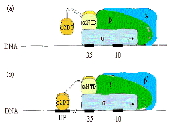
a. Recall from Part Three that the a subunit of RNA polymerase has two separate domains. The amino terminal domain (aNTD) is essential for dimerization and assembly of polymerase, and the carboxy terminal domain (aCTD) is needed for binding to DNA and for communication with many, but not all, transcription factors.

Most RNA polymerase (~60%) is associated with rRNA or tRNA genes. This is accomplished by a special sequence upstream of the promoter elements (i.e. the –35 and –10 boxes), called the UP element (-57)5'-AAAATTATTTT-3'(-47), which binds a2 dimers, and increases occupancy by polymerase by ~10-fold.

Fig. 4.2.12.

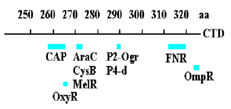
b. Much of the communication between activators and E. coli RNA polymerase is mediated between the CTD of a and these factors.

(see Ebright and Busby, 1995, Curr. Opinion in Gen. & Dev. 5:197-203)

Fig. 4.2.13.

3. Summary & Distinctions between Cap at Class I and Cap at Class II Promoters

(For reviews see Mol Micro 23:853-859 and Cur. Opin. Genet. Dev. 5:197-203).

Class I promoters have CAP binding sites centered at -62, -83, or -93.

At class II promoters, it is centered at -42 and overlaps the -35 determinant of the promoter.

Fig. 4.2.14. CAP binding to class I and class II promoters.

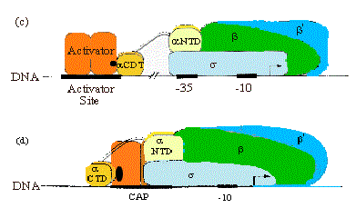
Legend to Fig. 4.2.14. The dimeric CAP protein is labeled "Activator". Binding to a class I promoter is shown in panel (c) and binding to a class II promoter is shown in panel (d).

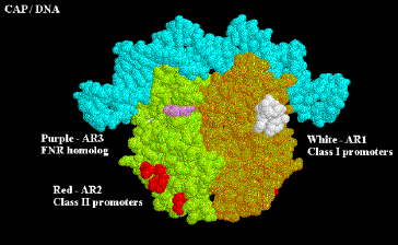
4. CAP has at least two Activation Regions (ARs):

• AR1 (residues 156-164)

At class I promoters, AR1 in the downstream subunit of CAP "sees" residues 258-265 of CTD of a. This interaction increases KB for polymerase binding to the promoter.

At class II promoters, CAP displaces the aCTD (decreasing KB), which is overcome by increasing KB via upstream subunit AR1-aCTD interaction

• AR2 (residues 19, 21, 96, 101)

At class II promoters, the downstream subunit "sees" aNTD residues 162-165, increasing kf for isomerization from closed to open complexes.

Fig. 4.2.15. Activation Regions on CAP

At both class I and class II promoters, CAP AR1 interacts with the CTD of a. It is clear that for class I promoters, residues 258-265 of the a subunit are the target of AR1 of CAP; it is not clear if these are the same residues needed for interaction at class II promoters. At class I promoters, this interaction provides "true" direct activation: the interaction is between the downstream subunit of CAP, and appears to only be used to increase KB for the binding of RNA polymerase to the promoter region (perhaps substituting for the lack of an UP sequence). At class II promoters, AR1 in the upstream subunit contacts the alpha subunit, but it does not appear to cause direct stimulation of transcription. Instead, it overcomes inhibition of polymerase that is hypothesized to arise from CAP displacing the alpha subunit from its preferred position near -45. This is evidenced by the following observations:

• aCTD binds to -40 to -55 region at class II promoters in the absence of CAP, but binds to the -58 to -74 region in its presence

• AR1 mutants in CAP decrease KB for RNA polymerase at class II promoters, but have no affect on kf .

• Removal of the a CDT eliminates the need for CAP AR1 in class II promoters, and has no negative affect.

• In contrast, removal of the a CDT prevents activation by CAP at class I promoters.

In addition to overcoming a decrease in KB by AR1, at class II promoters CAP also exerts a "direct" activation. This occurs between CAP residues 19, 21, 96 and 101 (AR2) in the downstream subunit of CAP, and residues 162-165 of the a subunit NTD. This interaction increases the kf and has no affect on KB. Region 162-165 is between regions 30-55 / 65-75 and 175-185 / 195-210 which are essential for contact with the b and b' subunits of polymerase, respectively. AR2 is not needed for CAP to work at class I promoters.

Appendix A for Chapter 17 (Part Four., section II)

Measurement of equilibrium constants for binding

of lac repressor to specific and nonspecific sites in DNA

R4 = Repressor

D S = Specific DNA site Þ operator

D NS = Nonspecific DNA site Þ all other sites in genome

R4 + DS R4DS R4 + DNS R4DNS

The lac repressor will bind to its specific site, the operator, with very high affinity,

Keq = KS = 2 x 1013 M-1, where Ks is the equilibrium association constant for binding to a specific site

and it will bind to other DNA sequences, or nonspecific sites, with a lower affinity.

Keq = KNS = 2 x 106 M-1, where Kns is the equilibrium association constant for binding to a nonspecific site.

Measurements in the laboratory:

Since it can be difficult to measure the amount of bound or free probe at very low concentrations, it is more reliable to measure the fraction of probe bound as a function of [R4]. The fraction of probe bound is

= .

By substituting [Ds] = [Ds]total - [R4Ds] into the equation for Ks, you can derive the following relationship between the fraction of probe bound by repressor and the concentration of the repressor:

=

{Since the [R4] is usually much greater than the [Ds]total in these assays, the

[R4]free >> [R4Ds], and [R4] is well approximated by [R4]total .}

This equation has the form of the classic Michaelis-Menten equation for steady-state enzyme kinetics, and it is also useful in analysis of many binding assays. Once is plotted against [R4], one can do curve fitting to derive a value for Ks. One can also get a value for Ks by measuring the [R4] at which half the probe is bound. At this point, [R4] = . {This can be seen simply by substituting = 0.5 into the equation above. The algebra is exactly the same as is done for the determination of Km by the Michaelis-Menten analysis.}

Appendix B. Use of binding constants and the equations relating the specificity parameter to the ratio of bound to free operator sites to study the effects of operator mutants.

The same equations used in section E of this chapter also can be used to examine the effects of operator mutants. The following analysis shows that a mutation that decreases the affinity of the operator 20-fold for the repressor will result in about half the operators being free of repressor (or the operon being expressed about half the time).

Specificity =

This says that the operator is essentially equally distributed between the bound and free form.

50% of the operators are not occupied by repressor, thus only about half of the operons will be expressed (in a population of bacteria), or any particular operon will be expressed about half the time.

Questions for Chapter 17. Transcriptional regulation by effects on RNA polymerase

16.1 The ratio [RDs]/[Ds] is the concentration of a hypothetical repressor (R) bound to its specific site on DNA divided by the concentration of unbound DNA, i.e. it is the ratio of bound DNA to free DNA. When the measured [RDs]/[Ds] is plotted versus the concentration of free repressor [R], the slope of the plot showed that the ratio [RDs]/[Ds] increased linearly by 60 for every increase of 1x10-11 M in [R]. What is the binding constant Ks for association of the repressor with its specific site?

16.2 The binding of the protein TBP to a labeled short duplex oligonucleotide containing a TATA box (the probe) was investigated quantitatively. The following table gives the fraction of total probe bound (column 2) and the ratio of bound to free probe (column 3) as a function of [TBP]. These data are provided courtesy of Rob Coleman and Frank Pugh.

[TBP] nM
0.10	0.040	0.042
0.20	0.16	0.19
0.30	0.33	0.5
0.40	0.44	0.78
0.50	0.52	1.1
0.70	0.62	1.6
1.0	0.71	2.45
2.0	0.83	4.88
3.0	0.87	6.69
5.0	0.93	14
10	0.97	32.3
20	0.99	99

Plot the data for the two different measures of bound probe. Note that since the denominator for column 2 is a constant, the ratio of bound to total probe will level off, whereas the amount of free probe can continue to decrease with increasing [TBP], and thereby getting a continuing increase in the ration of bound to free probe.

What is the equilibrium constant for TBP binding to the TATA box?

16.3 What is the fate of the lac repressor after it binds the inducer?

16.4 How does the lac repressor prevent transcription of the lac operon?

For the next two questions, let's imagine that you mixed increasing amounts of the DNA binding protein called AP1 with a constant amount of a labeled duplex oligonucleotide containing the binding site (TGACTCA). After measuring the fraction of DNA bound by AP1 (i.e. the fractional occupancy) as a function of [AP1], the data were analyzed by nonlinear, least squares regression analysis at a wide range of possible values for DG. The error associated with the fit of each of those values to experimental data is shown below; the higher the variance of fit, the larger the error.

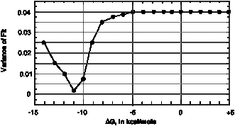
16.5 What is the most accurate value of DG for binding of AP1 to this duplex oligonucleotide?

16.6 What is the most accurate measure of the equilibrium constant, Ks, for binding of AP1 to this duplex oligonucleotide?

For the next two problems, consider a hypothetical eubacterial operon in which the operator overlaps the -10 region of the promoter. Measurement of the lag time before production of abortive transcripts (in an abortive initiation assay) as a function of the inverse of the RNA polymerase concentration (1/[RNAP]) gave the results shown below. The filled circles are the results of the assay in the absence of repressor, and the open circles are the results in the presence of repressor bound to the operator.

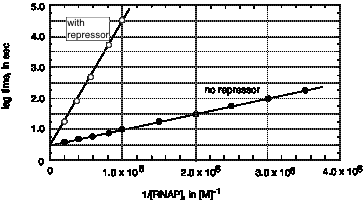
16.7 What is the value of the forward rate constant (kf ) for closed to open complex formation under the two different conditions?

16.8 What is the value of the equilibrium constant (KB ) for binding of the RNA polymerase to the promoter under the 2 conditions?