CHAPTER 4

GENOMES AND CHROMOSOMES

This chapter will cover:

§ Distinct components of genomes

§ Abundance and complexity of mRNA

§ Normalized cDNA libraries and ESTs

§ Genome sequences: gene numbers

§ Comparative genomics

§ Features of chromosomes

§ Chromatin structure

Sizes of genomes: The C‑value paradox

The C-value is the amount of DNA in the haploid genome of an organism. It varies over a very wide range, with a general increase in C-value with complexity of organism from prokaryotes to invertebrates, vertebrates, plants.

Figure 4.1.

The C-value paradox is basically this: how can we account for the amount of DNA in terms of known function?

Very similar organisms can show a large difference in C-value; e.g. amphibians.

The amount of genomic DNA in complex eukaryotes is much greater than the amount needed to encode proteins. For example:

Mammals have 30,000 to 50,000 genes, but their genome size (or C-value) is 3 x 109 bp.

(3 x 109 bp)/3000 bp (average gene size) = 1 x 106 (“gene capacity”).

Drosophila melanogaster has about 5000 mutable loci (~genes). If the average size of an insect gene is 2000 bp, then

>1 x 108 bp/2 x 103 bp = > 50,000 “gene capacity”.

Our current understanding of complex genomes reveals several factors that help explain the classic C-value paradox:

Introns in genes

Regulatory elements of genes

Pseudogenes

Multiple copies of genes

Intergenic sequences

Repetitive DNA

The facts that some of the genomic DNA from complex organisms is highly repetitive, and that some proteins are encoded by families of genes whereas others are encoded by single genes, mean that the genome can be considered to have several distinctive components. Analysis of the kinetics of DNA reassociation, largely in the 1970's, showed that such genomes have components that can be distinguished by their repetition frequency. The experimental basis for this will be reviewed in the first several sections of this chapter, along with application of hybridization kinetics to measurement of complexity and abundance of mRNAs. Advances in genomic sequencing have provided more detailed views of genome structure, and some of this information will be reviewed in the latter sections of this chapter.

Table 4.1. Distinct components in complex genomes

Highly repeated DNA

R (repetition frequency) >100,000

Almost no information, low complexity

Moderately repeated DNA

10<R<10,000

Little information, moderate complexity

“Single copy” DNA

R=1 or 2

Much information, high complexity

R = repetition frequency

Reassociation kinetics measure sequence complexity

Low complexity DNA sequences reanneal faster than do high complexity sequences

The components of complex genomes differ not only in repetition frequency (highly repetitive, moderately repetitive, single copy) but also in sequence complexity. Complexity (denoted by N) is the number of base pairs of unique or nonrepeating DNA in a given segment of DNA, or component of the genome. This is different from the length (L) of the sequence if some of the DNA is repeated, as illustrated in this example.

E.g. consider 1000 bp DNA.

500 bp is sequence a, present in a single copy.

500 bp is sequence b (100 bp) repeated 5 times:

a b b b b b

|___________|__|__|__|__|__| L = length = 1000 bp = a + 5b

N = complexity = 600 bp = a + b

Some viral and bacteriophage genomes have almost no repeated DNA, and L is approximately equal to N. But for many genomes, repeated DNA occupies 0.1 to 0.5 of the genome, as in this simple example.

The key result for genome analysis is that less complex DNA sequences renature faster than do more complex sequences. Thus determining the rate of renaturation of genomic DNA allows one to determine how many kinetic components (sequences of different complexity) are in the genome, what fraction of the genome each occupies, and the repetition frequency of each component.

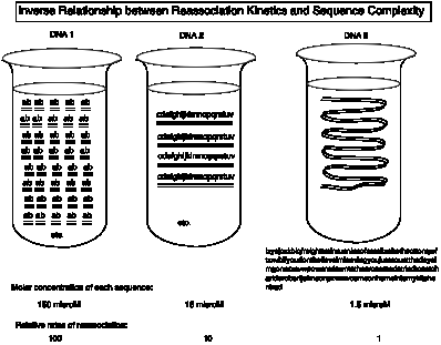
Before investigating this in detail, let's look at an example to illustrate this basic principle, i.e. the inverse relationship between reassociation kinetics and sequence complexity.

Illustration of the Inverse Relationship between Reassociation Kinetics and Sequence Complexity (see Fig. 4.2.)

Let a, b, ... z represent a string of base pairs in DNA that can hybridize. For simplicity in arithmetic, we will use 10 bp per letter.

DNA 1 = ab. This is very low sequence complexity, 2 letters or 20 bp.

DNA 2 = cdefghijklmnopqrstuv. This is 10 times more complex (20 letters or 200 bp).

DNA 3 = izyajczkblqfreighttrainrunninsofastelizabethcottonqwftzxvbifyoudontbelieveimleavingyoujustcountthedaysimgonerxcvwpowentdowntothecrossroadstriedtocatchariderobertjohnsonpzvmwcomeonhomeintomykitchentrad.

This is 100 times more complex (200 letters or 2000 bp).

A solution of 1 mg DNA/ml is 0.0015 M (in terms of moles of bp per L) or 0.003 M (in terms of nucleotides per L). We'll use 0.003 M = 3 mM, i.e. 3 mmoles nts per L. (nts = nucleotides).

Consider a 1 mg/ml solution of each of the three DNAs. For DNA 1, this means that the sequence ab (20 nts) is present at 0.15 mM or 150 mM (calculated from 3 mM / 20 nt in the sequence). Likewise, DNA 2 (200 nts) is present at 15 mM, and DNA 3 is present at 1.5 mM. Melt the DNA (i.e. dissociate into separate strands) and then allow the solution to reanneal, i.e. let the complementary strand reassociate.

Since the rate of reassociation is determined by the rate of the initial encounter between complementary strands, the higher the concentration of those complementary strands, the faster the DNA will reassociate. So for a given overall DNA concentration, the simple sequence (ab) in low complexity DNA 1 will reassociate 100 times faster than the more complex sequence (izyajcsk ....trad) in the higher complexity DNA 3. Fast reassociating DNA is low complexity.

Fig. 4.2.

Kinetics of renaturation

In this section, we will develop the relationships among rates of renaturation, complexity, and repetition frequency more formally.

Figure 4.3.

The time required for half renaturation is inversely proportional to the rate constant. Let C = concentration of single-stranded DNA at time t (expressed as moles of nucleotides per liter). The rate of loss of single-stranded (ss) DNA during renaturation is given by the following expression for a second-order rate process:

Integration and some algebraic substitution shows that

(1).

Thus, at half renaturation, when

one obtains:

(2)

where k is the rate constant in in liters (mole nt)-1 sec-1

The rate constant for renaturation is inversely proportional to sequence complexity. The rate constant, k, shows the following proportionality:

(3)

where L = length; N = complexity.

Empirically, the rate constant k has been measured as

in 1.0 M Na+ at T = Tm - 25oC

The time required for half renaturation (and thus Cot1/2 ) is directly proportional to sequence complexity.

From equations (2) and (3), (4)

For a renaturation measurement, one usually shears DNA to a constant fragment length L (e.g. 400 bp). Then L is no longer a variable, and

(5).

The data for renaturation of genomic DNA are plotted as C0t curves:

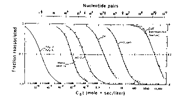
Figure 4.4.

Renaturation of a single component is complete (0.1 to 0.9) over 2 logs of C0t (e.g. 1 to 100 for E. coli DNA), as predicted by equation (1).

Sequence complexity is usually measured by a proportionality to a known standard.

If you have a standard of known genome size, you can calculate N from C0t1/2:

(6)

A known standard could be E. coli N = 4.639 x 106 bp or

pBR322 N = 4362 bp

More complex DNA sequences renature more slowly than do less complex sequences. By measuring the rate of renaturation for each component of a genome, along with the rate for a known standard, one can measure the complexity of each component.

Analysis of Cot curves with multiple components

In this section, the analysis in section B. is applied quantitatively in an example of renaturation of genomic DNA. If an unknown DNA has a single kinetic component, meaning that the fraction renatured increases from 0.1 to 0.9 as the value of C₀t increases 100-fold, then one can calculate its complexity easily. Using equation (6), all one needs to know is its C₀t_1/2 , plus the C₀t_1/2 and complexity of a standard renatured under identical conditions (initial concentration of DNA, salt concentration, temperature, etc.).

The same logic applies to the analysis of a genome with multiple kinetic components. Some genomes reanneal over a range of C₀t values covering many orders of magnitude, e.g. from 10^-3 to 10⁴. Some of the DNA renatures very fast; it has low complexity, and as we shall see, high repetition frequency. Other components in the DNA renature slowly; these have higher complexity and lower repetition frequency. The only new wrinkle to the analysis, however, is to treat each kinetic component independently. This is a reasonable approach, since the DNA is sheared to short fragments, e.g. 400 bp, and it is unlikely that a fast-renaturing DNA will be part of the same fragment as a slow-renaturing DNA.

Some terms and abbreviations need to be defined here.

f = fraction of genome occupied by a component

C0t1/2 for pure component = (f) (C0t1/2 measured in the mixture of components)

R = repetition frequency

G = genome size. G can be measured chemically (e.g. amount of DNA per nucleus of a cell) or kinetically (see below).

One can read and interpret the Cot curve as follows. One has to estimate the number of components in the mixture that makes up the genome. In the hypothetical example in Fig. 4.5, three components can be seen, and another is inferred because 10% of the genome has renatured as quickly as the first assay can be done. The three observable components are the three segments of the curve, each with an inflection point at the center of a part of the curve that covers a 100-fold increase in C₀t (sometimes called 2 logs of C₀t ). The fraction of the genome occupied by a component, f, is measured as the fraction of the genome annealing in that component. The measuredC₀t_1/2 is the value of C₀t at which half the component has renatured. In Fig. 4.5, component 2 renatures between C₀t values of 10^-3 and 10^-1, and the fraction of the genome renatured increased from 0.1 to 0.3 over this range. Thus f is 0.3-0.1=0.2. The C₀t value at half-renaturation for this component is the value seen when the fraction renatured reached 0.2 (i.e. half-way between 0.1 and 0.3; this C₀t value is 10^-2, and it is referred to as the C₀t_1/2 for component 2 (measured in the mixture of components). Values for the other components are tabulated in Fig. 4.5.

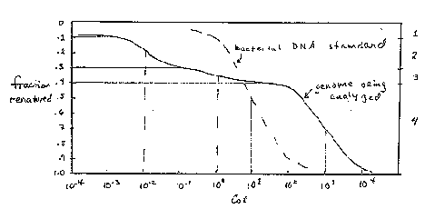
Figure 4.5.

All the components of the genome are present in the genomic DNA initially denatured. Thus the value for C₀ is for all the genomic DNA, not for the individual components. But once one knows the fraction of the genome occupied by a component, one can calculate the C₀ for each individual component, simply as C₀ ´ f. Thus the C₀t_1/2 for the individual component is the C₀t_1/2 (measured in the mixture of components) ´ f. For example the C₀t_1/2 for individual (pure) component 2 is 10^-2 ´ 0.2 = 2 ´ 10^-3 .

Knowing the measured Cot1/2 for a DNA standard, one can calculate the complexity of each component.

complexityn = Nn = C0t1/2pure, n ´

subscript n refers to the particular component, i.e. (1, 2, 3, or 4)

The repetition frequency of a given component is the total number of base pairs in that component divided by the complexity of the component. The total number of base pairs in that component is given by fn ´ G.

Rn =

For the data in Fig. 4.5, one can calculate the following values:

Component	f	C0t1/2 , mix	C0t1/2 , pure	N (bp)	R
1 foldback	0.1	< 10-4	< 10-4
2 fast	0.2	10-2	2 x 10-3	600	105
3 intermediate	0.1	1	0.1	3 x 104	103
4 slow (single copy)	0.6	103	600	1.8 x 108	1
std bacterial DNA			10	3 x 106	1

The genome size, G, can be calculated from the ratio of the complexity and the repetition frequency.

G =

E.g. If G = 3 x 108 bp, and component 2 occupies 0.2 of it, then component 2 contains 6 x 107 bp. But the complexity of component 2 is only 600 bp. Therefore it would take 105 copies of that 600 bp sequence to comprise 6 x 107 bp, and we surmise that R = 105.

Question 4.1.

If one substitutes the equation for Nn and for G into the equation for Rn, a simple relationship for R can be derived in terms of Cot1/2 values measured for the mixture of components . What is it?

Types of DNA in each kinetic component for complex genomes

Eukaryotic genomes usually have multiple components, which generates complex C0t curves. Fig. 4.6 shows a schematic C0t curve that illustrates the different kinetic components of human DNA, and the following table gives some examples of members of the different components.

Figure 4.6.

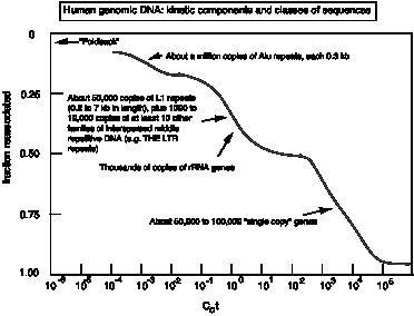
Table 4.2. Four principle kinetic components of complex genomes

Renaturation kinetics	C0t descriptor	Repetition frequency	Examples
too rapid to measure	"foldback"	not applicable	inverted repeats
fast renaturing	low C0t	highly repeated, > 105 copies per cell	interspersed short repeats (e.g. human Alu repeats); tandem repeats of short sequences (centromeres)
intermediate renaturing	mid C0t	moderately repeated, 10-104 copies per cell	families of interspersed repeats (e.g. human L1 long repeats); rRNA, 5S RNA, histone genes
slow renaturing	high C0t	low, 1-2 copies per cell, "single copy"	most structural genes (with their introns); much of the intergenic DNA

N, R for repeated DNAs are averages for many families of repeats. Individual members of families of repeats are similar but not identical to each other.

The emerging picture of the human genome reveals approximately 30,000 genes encoding proteins and structural or functional RNAs. These are spread out over 22 autosomes and 2 sex chromosomes. Almost all have introns, some with a few short introns and others with very many long introns. Almost always a substantial amount of intergenic DNA separates the genes.

Several different families of repetitive DNA are interspersed throughout the the intergenic and intronic sequences. Almost all of these are repeats are vestiges of transposition events, and in some cases the source genes for these transposons have been found. Some of the most abundant families of repeats transposed via an RNA intermediate, and can be called retrotransposons. The most abundant repetitive family in humans are Alu repeats, named for a common restriction endonuclease site within them. They are about 300 bp long, and about 1 million copies are in the genome. They are probably derived from a modified gene for a small RNA called 7SL RNA. (This RNA is involved in translation of secreted and membrane bound proteins.) Genomes of species from other mammalian orders (and indeed all vertebrates examined) have roughly comparable numbers of short interspersed repeats independently derived from genes encoding other short RNAs, such as transfer RNAs.

Another prominent class of repetitive retrotransposons are the long L1 repeats. Full-length copies of L1 repeats are about 7000 bp long, although many copies are truncated from the 5' end. About 50,000 copies are in the human genome. Full-length copies of recently transposed L1s and their sources genes have two open reading frames (i.e. can encode two proteins). One is a multifunctional protein similar to the pol gene of retroviruses. It encodes a functional reverse transcriptase. This enzyme may play a key role in the transposition of all retrotransposons. Repeats similar to L1s are found in all mammals and in other species, although the L1s within each mammalian order have features distinctive to that order. Thus both short interspersed repeats (or SINEs) and the L1 long interspersed repeats (or LINEs) have expanded and propogated independently in different mammalian orders.

Both types of retrotransposons are currently active, generating de novo mutations in humans. A small subset of SINEs have been implicated as functional elements of the genome, providing post-transcriptional processing signals as well as protein-coding exons for a small number of genes.

Other classes of repeats, such as L2s (long repeats) and MIRS (short repeats named mammalian interspersed repeats), appear to predate the mammalian radiation, i.e. they appear to have been in the ancestral eutherian mammal. Other classes of repeats are transposable elements that move by a DNA intermediate.

Other common interspersed repeated sequences in humans

LTR-containing retrotransposons

MaLR: mammalian, LTR retrotransposons

Endogenous retroviruses

MER4 (MEdium Reiterated repeat, family 4)

Repeats that resemble DNA transposons

MER1 and MER2

Mariner repeats

Some of the repeats are clustered into tandem arrays and make up distinctive features of chromosomes (Fig. 4.7). In addtion to the interspersed repeats discussed above, another contributor to the moderately repetitive DNA fraction are the thousands of copies of rRNA genes. These are in extensive tandem arrays on a few chromosomes, and are condensed into heterochromatin. Other chromosomal structures with extensive arrays of tandem repeats are centromeres and telomeres.

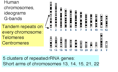
Figure 4.7. Clustered repeated sequences in the human genome.

The common way of finding repeats now is by sequence comparison to a database of repetitive DNA sequences, RepBase (from J. Jurka). One of the best tools for finding matches to these repaats is RepeatMasker (from Arian Smit and P. Green, U. Wash.). A web server for RepeatMasker can be accessed at:

http://ftp.genome.washington.edu/cgi-bin/RepeatMasker

Question 4.2. Try RepeatMasker on INS gene sequence. You can get the INS sequence either from NCBI (GenBank accession gi|307071|gb|L15440.1 or one can use LocusLink, query on ) or from the course website.

Very little of the nonrepetive DNA component is expressed as mRNA

Hybridization kinetic studies of RNA revealed several important insights. First, saturation experiments, in which an excess of unlabeled RNA was used to drive labeled, nonrepetitive DNA (tracer) into hybrid, showed that only a small fraction of the nonrepetitive DNA was present in mRNA. Classic experiments from Eric Davidson’s lab showed that only 2.70% of total nonrepetitive DNA correspondss to mRNA isolated from sea urchin gastrula (this is corrected for the fact that only one strand of DNA is copied into RNA; the actual amount driven into hybrid is half this, or 1.35%; Fig. 4.8). The complexity of this nonrepetitive fraction is (Nsc ) is 6.1 x 108 bp, so only 1.64 x 107 bp of this DNA is present as mRNA in the cell. If an "average" mRNA is 2000 bases long, there are ~8200 mRNAs present in gastrula.

In contrast, if the nonrepetitive DNA is hybridized to nuclear RNA from the same tissue, 28% of the nonrepetitive fraction corresponds to RNA (Fig. 4.8). The nuclear RNA is heterogeneous in size, and is sometimes referred to as heterogeneous nuclear RNA, or hnRNA. Some of it is quite large, much more so than most of the mRNA associated with ribosomes in the cytoplasm. The latter is called polysomal mRNA.

Figure 4.8.

Figure 4.8.

These data show that a substantial fraction of the genome (over one-fourth of the nonrepetitive fraction) is transcribed in nuclei at the gastrula stage, but much of this RNA never gets out of nucleus (or more formally, many more sequences from the DNA are represented in nuclear RNA than in cytoplasmic RNA). Thus much of the complexity in nuclear RNA stays in the nucleus; it is not processed into mRNA and is never translated into proteins.

Factors contributing to an explanation include:

1. Genes may be transcribed but the RNA is not stable. (Even the cytoplasmic mRNA from different genes can show different stabilities; this is one level of regulation of expression. But there could also be genes whose transcripts are so unstable in some tissues that they are never processed into cytoplasmic mRNA, and thus never translated. In this latter case, the gene is transcribed but not expressed into protein.)

2. Intronic RNA is transcribed and turns over rapidly after splicing.

3. Genes are transcribed well past the poly A addition site. These transcripts through the 3' flanking, intergenic regions are usually very unstable.

4. Not all of this "extra" RNA in the nucleus is unstable. For instance, some RNAs are used in the nucleus, e.g.:

U2-Un RNAs in splicing (small nuclear RNAs, or snRNAs).

RNA may be a structural component of nuclear scaffold (S. Penman).

Thus, although 10 times as much RNA complexity is present in the nucleus compared to the cytoplasm, this does not mean that 10 times as many genes are being transcribed as are being translated. Some fraction (unknown presently) of this "excess" nuclear RNA may represent genes that are being transcribed but not expressed, but many other factors also contribute to this phenomenon.

mRNA populations in different tissues show considerable overlap:

Housekeeping genes encode metabolic functions found in almost all cells.

Specialized genes, or tissue-specific genes, are expressed in only 1 (or a small number of) tissues. These tissue-specific genes are sometimes expressed in large amounts.

Estimating numbers of genes expressed and mRNA abundance from the kinetics of RNA-driven reactions

Using principles similar to those for analysis of repetition classes in genomic DNA, one can determine from the kinetics of hybridization between a preparation of RNA and single copy DNA both the average number of genes represented in the RNA, as well as the abundance of the mRNAs. The details of the kinetic analysis will not be presented, but they are similar to those already discussed. Highly abundant RNAs (like high copy number DNA) will hybridize to genomic DNA faster than will low abundance RNA (like low copy number DNA). Only a few mRNAs are highly abundant, and they constitute a low complexity fraction. The bulk of the genes are represented by lower abundance mRNA, and these many mRNAs constitute a high complexity, slowly hybridizing fraction.

An example is summarized in Table 4.3. an excess of mRNA from chick oviduct washybridized to a tracer of labeled cDNA (prepared from oviduct mRNA). Three principle components were found, ranging from the highly abundant ovalbumin mRNA to much rarer mRNAs from many genes.

Table 4.3.

Component	Kinetics of hybridization	N (nt)	# mRNAs	Abundance	Example
1	fast	2,000	1	120,000	Ovalbumin
2	medium	15,000	7-8	4,800	Ovomucoid, others
3	slow	2.6 x 107	13,000	6-7	Everything else

Preparation of normalized cDNA libraries for ESTs

Just like the mRNA populations used as the templates for reverse transcriptase, the cDNAs from a particular tissue or cell type will be composed of many copies of a very few, abundant mRNAs, a fairly large number of copies of the moderately abundant mRNAs, and a small number of copies of the rare mRNAs. Since most genes produce low abundance mRNA, a corresponding small number of cDNAs will be made from most genes. In an effort to obtain cDNAs from most genes, investigators have normalized the cDNA libraries to remove the most abundant mRNAs.

The cDNAs are hybridized to the template mRNA to a sufficiently high Rot (concentration of RNA ´ time) so that the moderately abundant mRNAs and cDNAs are in duplex, whereas the rare cDNAs are still single-stranded. The duplex mRNA-cDNA will stick to a hydroxyapatite column, and the desired single-stranded, low abundance cDNA will elute. This procedure can be repeated a few times to improve the separation. The low abundance, high complexity cDNA is then ligated into a cloning vector to construct the cDNA library.

This normalization is key to the success of a random sequencing approach. Random cDNA clones, hundreds of thousands of them, have been picked and sequenced. A single-pass sequence from one of these cDNA clones is called an expressed sequence tag, or EST (Fig. 4.9). It is called a “tag” because it is a sequence of only part of the cDNA, and since it is in cDNA, which is derived from mRNA, it is from an expressed gene. If the cDNA libraries reflected the normal abundance of the mRNAs, then this approach would result in re-sequencing the abundant cDNAs over and over, and most of the rare cDNAs would never be sequenced. However, the normalization has been successful, and many genes, even with rare mRNAs, are represented in the EST database.

As of May, 2001, over 2,700,000 ESTs individual sequences of human cDNA clones have been deposited in dbEST. They are grouped into nonredundant sets (called Unigene clusters). Over 95,000 Unigene clusters have been assembled, and almost 20,000 of them contain known human genes. The estimated number of human genes is less than the number of Unigene clusters, presumably because some large genes are still represented in more than one Unigene cluster. It is likely that most human genes are represented in the EST databases. Exceptions include genes expressed only in tissues which have not been sampled in the cDNA libraries. For more information, see http://www.ncbi.nlm.nih.gov/UniGene/index.html

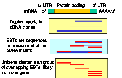
Figure 4.9. cDNA clones from normalized libraries are sequenced to generate ESTs.

H. Genome analysis by large scale sequencing

1. Whole genomes can be sequenced both by random shot-gun sequencing and by a directed approach using mapped clones.

A seminal advance from J. Craig Venter and his colleagues at The Institute for Genome Research in 1995 heralded a new era in genome analysis. They reported the complete sequence of the genome of the bacterium Haemophilus influenza , all 1,830,137 bp (Fleischmann et al., Science, vol. 269, pp. 496-512, 1995). In this method, genomic DNA is randomly sheared into small fragments about 1000 bp in size, cloned into plasmids, and determining the sequence from the ends of randomly picked clones (Fig. 4.10). This process is repeated many times, until each nucleotide in the genome has been sequenced multiple times on average. If the genome is 3 million base pairs, then determining 9 million base pairs of sequence from random clones give 3X coverage of the genome. This is sufficient data from which an almost-complete sequence of a bacterial genome can be assembled by linking overlapping sequences, using computational tools. Some gaps remain, and these are filled with directed sequencing. Larger genomes can be sequenced (or at least a major portion of them) by going to higher coverage, e.g. 8X to 10X. This approach requires NO prior knowledge of the genes or their positions on the bacterial chromosome. Several bacterial genomes have been sequenced this way, and Dr. Venter and colleagues have used the same approach to sequence almost all of the genomes of Drosophila melanogaster (in a collaboration between his company Celera and a publicly funded effort) and Homo sapiens (in a competition with the publicly funded effort). Variations on this theme improve effectiveness, such as cloning and sequencing both small (1 kb) and large (10 kb) inserts into plasmids, and then using the sequences from the ends of the longer inserts to help assemble the overall sequence. A similar idea uses the sequence from the ends of BAC inserts, which are about 100 kb in size, for large-scale assembly.

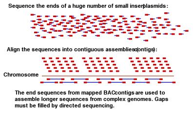
Figure 4.10. Shotgun sequencing and assembly.

Other major genome sequencing projects, such as those that generated the Saccharomyces cerevisiae and E. coli sequences, started with a large set of mapped clones, which were then sequenced in a directed manner. This works well, and one has a high resolution genetic and physical map for years before the genome sequence is complete. It is slower than the random approach, but it may achieve a greater extent of completeness for large, complex genomes. This is essentially the approach that the publicly funded, international collaboration, referred to as the International Human Genome Sequencing Consortium (IHGSC), followed.

The most recent phase of this project made extensive use of BAC clones, with an average insert size of about 100 kb (Fig. 4.11). Libraries of BAC clones containing human DNA inserts were ordered by a high throughput mapping effort. Restriction digests of each clone in the library were analyzed, and overlapping clones determined by finding fragments in common. The BAC clones were then organized into contiguous overlapping arrays, or contigs. A minimal tiling path needed to determine the sequence of each chromosome was established, and the ends of the BAC clones on that path were sequenced to provide a dense array of markers through the chromosome. BAC clones in the contigs were then sequenced, at this point using the shotgun sequencing of the BAC insert (100 kb), not the whole genome (3.2 million kb). Sequences of BAC clones at about 3X coverage are called draft sequences, and those at higher coverage with gaps filled by directed sequencing are considered finished sequences. A combination of draft and finished sequence data are being assembled using the BAC end sequences and other information. The assembly is publicly available at the Human Genome Browser at the University of California at Santa Cruz (http://genome.ucsc.edu/goldenPath/hgTracks.html) and the Ensembl site at the Sanger Center (http://www.ensembl.org/).

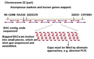
Figure 4.11. Directed sequencing of BAC contigs.

The results of the Celera and public collaboration on the fly sequence was published in early 2000, and descriptions of the human genome sequence were published separately by Celera and IHGSC in 2001. Neither genome is completely sequenced (as of 2001), but both are highly sequenced and are stimulating a major revolution in the life sciences.

The wisdom of which approach to take is still a matter of debate, and depends to some extent on how thoroughly one needs to sequence a complex genome. For instance, a publicly accessible sequence of the mouse genome at 3X coverage was recently generated by the shotgun approach. Other genomes will likely be “lightly sequenced” at a similar coverage. But a full, high quality sequence of mouse will likely use aspects of the more directed approach. Also, the Celera assembly (primarily shotgun sequence) used the public data on the human genome sequence as well. Thus current efforts use both the rapid sequencing by shotgun methods and as well as sequencing mapped clones.

Survey of sequenced genomes

The genome sequences are available for many species now, covering an impressive phylogenetic range. This includes more than 28 eubacteria, at least 6 archaea, a fungus (the yeast Saccharomyces cerevisiae), a protozoan (Plasmodium falciparum), a worm (the nematode Caenorhabditis elegans), an insect (the fruitfly Drosophila melanogaster), two plants (Arabadopsis and rice (soon)), and two mammals (human Homo sapiens and mouse Mus domesticus). Some information about these is listed in Table 4.4.

Table 4.4. Sequenced genomes. This table is derived from the listing of “Complete Genomes Mapped on the KEGG Pathways (Kyoto Encyclopedia of Genes and Genomes)” at

http://www.genome.ad.jp/kegg/java/org_list.html

Additional genomes have been added, but only samples of the bacterial sequences are listed.

Genes encoding

Species	Genome Size (bp)	Protein	RNA	Total Enzymes	Category
Eubacteria
Escherichia coli	4,639,221	4,289	108	1,254	gram negative
Haemophilus influenzae	1,830,135	1,717	74	571	gram negative
Helicobacter pylori	1,667,867	1,566	43	394	gram negative
Bacillus subtilis	4,214,814	4,100	121	819	gram positive
Mycoplasma genitalium	580,073	467	36	202	gram positive
Mycoplasma pneumoniae	816,394	677	33	226	gram positive
Mycobacterium tuberculosis	4,411,529	3,918	48	-	gram positive
Aquifex aeolicus	1,551,335	1,522	50	-	hyperthermophilic bacterium
Borrelia burgdorferi	1,230,663	1,256	23	176	lyme disease Spirochete
Synechocystis sp.	3,573,470	3,166	49	702	cyanobacterium
Archaebacteria
Archaeoglobus fulgidus	2,178,400	2,407	49	439	S-metabolizing archaea
Methanococcus jannaschii	1,739,934	1,735	43	441	archaea
Methanobacterium thermoautotrophicum	1,751,377	1,871	47	558	archaea
Eukaryotes
Saccharomyces cerevisiae	12,069,313	6,064	262	861	fungi
Caenorhabditis elegans	97,000,000	18,424		-	nematode
Drosophila melanogaster	180,000,000	13,601			insect, fly, 120 Mb sequenced
Arabidopsis thaliana	115,500,000	25,706			plant, complete
Homo sapiens	3,200,000,000	30,000-40,000			human, draft + finished
Mus domesticus	3,000,000,000				mouse, draft

Genome size.

Bacterial genomes range in size from 0.58 to almost 5 million bp (Mb). E. coli and B. subtilis, two of the most intensively studied bacteria, have the largest genomes and largest numbers of genes. The genome of the yeast Saccharomyces cerevisiae is only 2.6 times as large as that of E. coli. The genome of humans is almost 700 times larger than that of E. coli. However, genome size is not a direct measure of genetic content over long phylogenetic distances. One needs to examine the fraction of the genome that codes for protein or contains other important information. Let’s look at sizes and numbers of genes in different genomes.

Gene size and number.

The average gene size is similar among bacteria, averaging around 1100 bp. Very little DNA separates most bacterial genes; in E. coli there is an average of only 118 bp between genes. Since the gene size varies little, then the number of genes varies over as wide a range as the genome size, from 467 genes in M. genitalium to 4289 in E. coli. Thus within bacteria, which have little noncoding DNA, the number of genes is proportional to the genome size.

Saccharomyces cerevisiae has one gene every 1900 bp on average, which could reflect both an increase in size of gene as well as somewhat greater distance between genes. Both bacteria and yeast show a much denser packing of genes than is seen in more complex genomes.

Data on a large sample of human genes shows that they are much larger than bacterial genes, with the median being about 14 times larger than the 1 kb bacterial genes. This is not because most human proteins are substantially larger; both bacterial proteins average about 350 amino acids in length, which is similar to the median size of human proteins. The major difference is the large amount of intronic sequence in human genes.

Table 4.5. Average size of human genes and parts of genes. This is based on information in the IHGSC paper in Nature, and derived from analysis of 1804 human genes.

	Median	Mean
Internal exon	122 bp	145 bp
Number of exons	7	8.8
Length of each intron	1023 bp	3365 bp
3’ UTR	400 bp	770 bp
5’ UTR	240 bp	300 bp
Coding sequence	1100 bp	1340 bp
Length of protein encoded	367 amino acids	447 amino acids
Genomic extent	14,000 bp	27,000 bp

Summary of average gene size:

Bacteria: 1100 bp

Yeast: ~1200 bp

Worm: ~5000 bp

Human: ~27,000 bp

A comparison of the distribution of sizes of introns and exons show considerable overlap for worms, flies and humans. However, humans have a smaller fraction of long exons and a larger frction of long introns (Fig. 4.12).

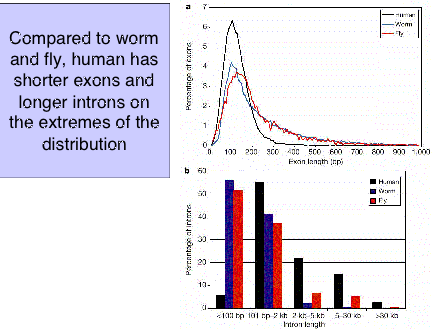
Figure 4.12. Distribution of exon and intron length in worms, fly and humans. From the IHGSC paper on the initial analysis of the human genome.

Distance between genes

Summary of distance between genes:

Bacteria: 118 bp

Yeast: ~700 bp

Human: may be about 10,000 bp

The distance between genes differs greatly between larger and smaller genomes. Genes are very close together in bacteria (about 100 bp), and much of that intergenic DNA appears to be involved in regulation. In yeast, the genes are 6 times further apart. In mammals, an enormouse expansion in the amount of DNA between genes is seen. Precise numbers await more complete annotation of the human sequence, but many examples are known of adjacent genes that are separated by 10 to 50 kb of nongenic DNA. In all these species, some DNA sequences regulating expression of genes are found in these intergenic spaces, but it is unlikely that all of this is required for regulation in mammals. Deciphering the important from the expendable sequences in intergenic sequences is a major current challenge. This applies to noncoding DNA in general

The number of genes per length of the chromosome is a reflection of the size of the genes and the distances between them. This gene density varies little in bacteria and yeast, but it changes over a wide range in various regions of the human genome. A higher gene density correlates with higher G+C content of a region (Fig. 4.13)

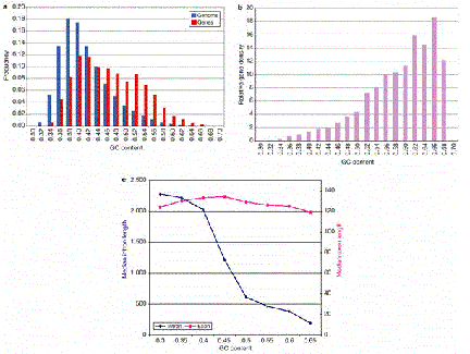
Figure 4.13. Higher G+C content correlates with higher gene density and shorter introns.

Genome size increases exponentially, but not number of genes

Table 4.4. documents a 5500-fold increase in genome size from the smallest bacterial genome to that of human. However, this is accompanied by only a roughly 65-fold increase in the number of genes. This trend is seen over the known range of genomic sequences. The genome size increases exponentially as one examines species covering the range of complexity from bacteria to humans (Fig. 4.14). However, the numbe of genes increases linearly. The plot in Fig. 4.14 was based on earlier, higher estimates for the number of genes in humans. The effect is even more pronounced if one uses 30,000 as the number of human genes.

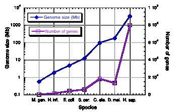
Figure 4.14. Genome size and number of genes in species ranging from bacteria to humans.

Alternative splicing is common in human genes

A previous lower estimate is that alternative splicing occurs in 35% of human genes. However, recent data show this fraction is larger.

For Chromosome 22:

642 transcripts cover 245 genes, 2.6 txpts/gene

2 or more transcripts for 145 (59%) of genes

For Chromosome 19:

1859 transcripts cover 544 genes, 3.2 txpts/gene

This contrasts with the situation in worm, in which alternative splicing occurs in 22% of genes.

The increased genetic diversity from alternative splicing may contribute considerably to the greater complexity of humans, not just the increase in the number of genes.

Estimates of number of human genes

The estimated number of human genes has varied greatly over recent years. Some of these numbers have been widely quoted, and it may be useful to list some of the sources of these estimates.

mRNA complexity (association kinetics): 40,000 genes

Avg size of gene 30,000 bp: 100,000 genes

Number of CpG islands: 70,000 to 80,000

Unigene clusters of ESTs: 35,000 to 125,000

More rigorous EST clustering: 35,000 genes

Comparison to pufferfish: 30,000 genes

Extrapolate from gene counts on chromosomes 21 and 22 (which are finished): 30,000 to 35,500 genes

Using the draft human sequence from Juy 2000, the IHGSC constructed an Initial Gene Index for human. They use the Ensembl system at the Sanger Centre. They started with ab initio predictions by Genscan, then confirmed by similarity to proteins, mRNAs, ESTs, and protein motifs (Pfam database) from any organism. This led to an initial set of 35,500 genes and 44,860 transcripts in the Ensemble database. After reducing fragmentation, merging with known genes, and removing contaminating bacterial sequences, they were left with 31,778 genes. After taking into account residual fragmentation, and the rate at which true genes are found by a similar analysis, the estimate remains about 32, 000 genes. However, it is an estimate and is subject to change as more annotation is completed..

Starting with this estimate that the human genome contains about 32,000 genes, one can calculate how much of the genome is coding and how much is transcribed. If the average coding length is 1400 bp, then 1.5% of human genome consists of coding sequence. If the average genomic extent per gene is 30 kb, then 33% of human genome is “transcribed”.

Summary of number of genes in eukaryotic species:

Human: 32,000 “still uncertain”

Fly: 13, 338

Worm: 18,266

Yeast: 6,144

Mustard weed: 25,706

Human: 2x number of genes in fly and worm

Human: more alternative splicing, perhaps 5x number of proteins as in fly or worm

Assignment of functions to genes.

Genes encoding proteins and RNAs can be detected with considerable accuracy using compuational tools. Note that even for an extensively studies organism like E. coli, the number of genes found by sequence analysis (4289 encoding proteins) is far greater than the number that can be assigned as encoding a particular enzyme (1254). The discrepancy between genes found in the sequence versus those with known function (i.e. assigned as encoding an enzyme) is greater for some poorly characterized organisms such as the lyme-disease causing Spirochete Borrelia burgdorferi.

The many genes with unassigned function present an exciting challenge both in bioinformatics and in biochemistry/cell biology/genetics. Large collaborations have been initiated for a comprehensive genetic and expression analysis of some organisms. For instance, projects are underway to make mutations in all detected genes in Saccharomyces cerevisiae and to quantify the level of stable RNA from each gene in a variety of growth conditions, through the cell cycle and in other conditions. Databases are already established that record the changes in RNA levels for all yeast genes when the organism is shifted from glucose to galactose as a carbon source. These large scale expression analysis use high density microchip arrays that contain characteristic sequences for all 6064 yeast genes. These gene arrays are then hybridized with fluorescently labeled RNA or cDNA from cells grown under the two different conditions. The hybridization signals are quantitated and compared automatically, analyzed. The plan is to store the results in public databases. Useful websites include:

SGD at http://genome-www.stanford.edu/Saccharomyces/

mips at http://speedy.mips.biochem.mpg.de/mips/yeast/index.htmlx

Databases for genomic analysis

NCBI

http://www.ncbi.nlm.nih.gov

Nucleic acid sequences

genomic and mRNA, including ESTs

Protein sequences

Protein structures

Genetic and physical maps

Organism-specific databases

MedLine (PubMed)

Online Mendelian Inheritance in Man (OMIM)

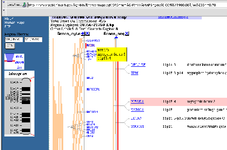
Figure 4.15. Example of mapping information at NCBI. Genetic map around MYOD1, 11p15.4

Sequences and annotation of the human genome

Human Genome Browser

http://genome.ucsc.edu/goldenPath/hgTracks.html

Ensemble (European Bioinformatics Institute (EMBL) and Sanger Centre)

http://www.ensembl.org/

A.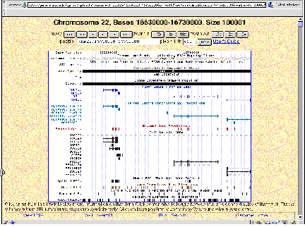

B.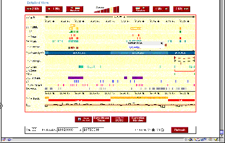

Figure 4.16. Sample views from servers displaying the human genome. (A) View from the Human Genome Browser. The region shown is part of chromosome 22 with the genes PNUTL1, TBX1 and others. Extensive annotation for exons, repeats, single nucleotide polymorphisms, homologous regions in mouse and other information is available for all the sequenced genome. (B) Comparable information in a different format is available at the ENSEMBL server.

Programs for sequence analysis

BLAST to search rapidly through sequence databases

PipMaker (to align 2 genomic DNA sequences)

Gene finding by ab initio methods (GenScan, GRAIL, etc.)

RepeatMasker

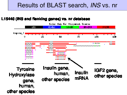
Figure 4.18. Results of BLAST search, INS vs. nr

Large scale genome organization

How to get by with the smallest possible genome.

The Mycoplasma species have the smallest genomes of any free-living species. They are most related to the Bacillaceae family, but have lost their cell walls and many other functions in a process of reductive evolution. They are obligate parasites, e.g. living in the lungs of humans. Their genomes encode many transport proteins, so that amino acids, sugars, etc. can be taken up from their hosts. They have very little metabolic capacity, utilizing only glycolysis in the case of M. genitalium. There is very little biosynthetic capacity, depending largely on uptake from the host for these nutrients.

One might have thought that the Mycoplasmal species would retain only the most highly conserved genes in bacteria, under the premise that these are the most critical genes. However, they have retained a proportion of conserved and variable genes that is quite similar to the proportion seen in E. coli. This indicates that these bacteria are maintaining a balance between conserved and variable genes that perhaps reflects an equilibrium between the stability of major physiological processes and the need for environmental adaptability.

More information from E. coli

The complete sequence of the E. coli genome provides an overview of genome structure within a well-understood context. For more information, see Blattner et al. (1997) Science, vol. 277, pp. 1453- 1462.

Organization with respect to direction of replication.

Since replication proceeds bidirectionally from the origin (oriC) and ends at the terminus, one can divide the genome into two "replicores." The replication fork proceeds clockwise in Replicore 1 and counter-clockwise in Replicore 2 (Fig. 4.19).

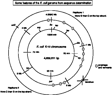
Figure 4.19.

Several features of the genome are oriented with respect to replication. All the rRNA genes, 53 of 86 tRNA genes, and 55% of the protein coding genes are transcribed in the same direction as the replication fork moves. In other species, such as the Mycoplasma, the transcriptional polarity is even more pronounced, and it also corresponds to the direction of replication.

These replicores show a pronounced skew in base composition, such that an excess of G over C is seen on the top strand (i.e. the one presented in the sequence file) in Replicore 1 and the opposite in Replicore 2. This nucleotide bias is striking and unexpected. As will be appreciated more after we study DNA synthesis in Part Two, this means that the leading strand for both replication forks is richer in G than C. Such an nucleotide bias may reflect differential mutation in the leading and lagging strands as a result of the asymmetry inherent in the DNA replication mechanism.

The recombination hotspot chi (GCTGGTGG) also shows a prominent strand preference, being more abundant on the leading strand of each replicore. The role of chi sites in recombination is covered in Chapter 8.

(2) Repeats, prophage and transposable elements.

The E. coli chromosome contains several prophages and remnants of prophage, including lambda and three lambdoid prophages. The genome is peppered with at least 18 families of repeated DNA. The longest are the 5 Rhs elements, which are 5.7 to 9.6 kb in length. Others are as short as the 581 copies of the 40 bp palindromic REP repeat. Several families of insertion sequences, which are transposable elements, are found. Note that repetitive elements are common in bacteria as well as in eukaryotes.

(3) General categories of genes.

Many of the genes are similar to other genes in E. coli. Homologous genes that have diverged because of gene duplications are paralogous. The genes that encode proteins of similar but not necessarily identical function are referred to as a paralogous family. About 1/3 of the E. coli genes (1345) have at least one paralogous sequence in the genome. Some paralogous groups are quite large, the largest being the ABC transporters with 80 members. The larger number of genes in E. coli could reflect some redundancy in function as well as greater diversification of function compared to other bacteria with fewer genes.

Based on current understanding of the function of the gene products, about 1/4 are involved in small-molecule metabolism, about 1/8 are used in large-molecule metabolism, and at least 1/5 are associated with cell structure and processes. A specific function has not been assigned to the products of about 40% of the E. coli genes.

Human: Multiple chromosomes

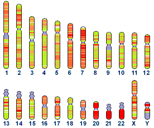
Figure 4.20. Human chromosomes, and the status of their sequencing.

http://www.ncbi.nlm.nih.gov/genome/seq/

Segmental duplications are common, as illustrated in Fig. 4.21 for chromosomes 22.

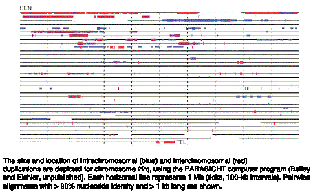
Figure 4.21. Segmental duplications on chromosome 22.

Comparative Genome Analysis

Paralogous genes

Genes that are similar because of descent from a common ancestor are homologous.

Homologous genes that have diverged after speciation are orthologous.

Homologous genes that have diverged after duplication are paralogous.

One can identify paralogous groups of genes encoding proteins of similar but not identical function in a species

E.g. ABC transporters: 80 members in E. coli

Core proteomes vary little in size

Proteome: all the proteins encoded in a genome

To calculate the Core proteome:

Count each group of paralogous proteins only once

Number of distinct protein families in each organism

Species Number of genes Core proteome

Haemophilus 1709 1425

Yeast 6241 4383

Worm 18424 9453

Fly 13601 8065

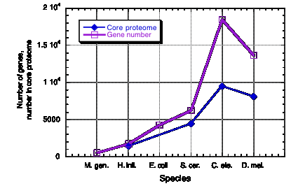
Figure 4.22. Little change in core proteome size in eukaryotes

Core proteomes are conserved

Many of the proteins in the core proteomes are shared among eukaryotes

30% of fly genes have orthologs in worm

20% of fly genes have orthologs in both worm and yeast

50% of fly genes have likely orthologs in mammals

Function of proteins in flies (and worms and yeast) provides strong indicators of function in humans

Flies have orthologs to 177 of the 289 human disease genes

Figure 4.23. Functional categories in eukaryotic proteomes

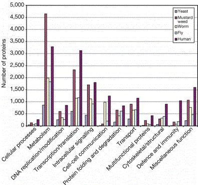
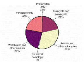
Figure 4.24. Distribution of the homologues of the predicted human proteins

Conserved segments in the human and mouse genomes

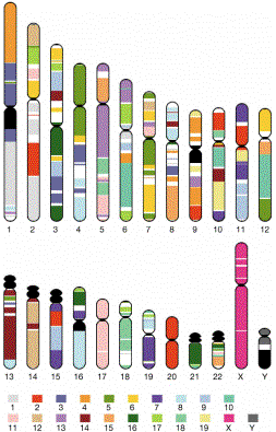
Figure 4.25. Regions of human chromosomes homologous to regions of mouse chromosomes (indicated by the colors). For example, virtually all of human chromosome 20 is homologous to a region on mouse chromosome 2, and almost all of human chromosome 17 is homologous to a region on mouse chromosome 11. More commonly, segments of a given human chromosomes are homologous to different mouse chromosomes. Chromsosomes from mouse have more rearrangements relative to humans than do chromosomes from many mammals, but the homologous relationships are still readily apparent.

CHROMOSOMES AND CHROMATIN

Chromosomes are the cytological package for genes

Genomes are much longer than the cellular compartment they occupy

compartment dimensions length of DNA

Phage T4 0.065x0.10 mm 55 mm = 170 kb

E. coli 1.7x0.65 mm 1.3 mm = 4.6x103 kb

Nucleus (human) 6 mm diam. 1.8 m = 6x106 kb

Packing ratio = length of DNA / length of the unit that contains it.

E.g. smallest human chromosome contains about 46 ´ 106 bp = 14,000 mm = 1.4 cm DNA. When condensed for mitosis, this chromosome is about. 2 mm long. The packing ratio is therefore about 7000!

Loops, matrix and the chromosome scaffold

When DNA is released from mitotic chromosomes by removing most of the proteins, long loops of DNA are seen, emanating from a central scaffold that resembles the remnants of the chromosome.

Figure 4.26.

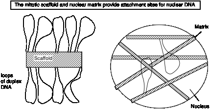
EM analysis of intact nuclei shows network of fibers called a matrix.

Biochemical preparations using salt and detergent to remove proteins and nuclease to remove most of the DNA leaves a "matrix" or "scaffold" preparation. Similar DNA sequences are found in these preparations; these sequences are called matrix attachment regions = MARs (or scaffold attachment regions = SARs). They tend to be A+T rich and have sites for cleavage by topoisomerase II. Topoisomerase II is one of the major components of the matrix preparation; but the composition of the matrix is still in need of further study.

Since it is attached at the base to the matrix, each loop is a separate topological domain and can accumulate supercoils of DNA.

From the measured sizes of loops, and calculations based on the amount of nicking required to relax DNA within the loops, we estimate that the average size of these loops is about 100 kb (85 kb based on nicking frequency for relaxation).

Some evidence suggests that replication and possibly some transcriptional control may be exerted at the bases of the loops.

Interphase chromatin and mitotic chromosomes

During interphase, i.e. between mitotic divisions, the highly condensed mitotic chromosomes spread out through the nucleus to form chromatin. Interphase chromatin is not very densely packed in most of the nucleus (euchromatin). In some regions it is very densely packed, comparable to a mitotic chromosome (heterochromatin).

Both interphase chromatin and mitotic chromosomes are made of a 30 nm fiber. The mitotic chromosome is much more coiled than interphase chromosomes.

Most transcription occurs in euchromatin.

Constitutive heterochromatin = nonexpressed regions that are condensed (compact) in all cells (e.g. centromeric simple repeats)

Facultative heterochromatin = inactive in only some cell lineages, active in others.

One example of heterochromatin is the inactive X chromosome in female mammals. The choice of which X chrosomosome to inactivate is random in various cell lineages, leading to a mosaic phenotypes for some X-linked traits. For instance, one genetic determinant of coat color in cats is X-linked, and the patchy coloration on calico cats results from this random inactivation of one of the X chromosomes, leading to the lack of expression of this determinant in some but not all hair cells.

Cytologically visible bands in chromosomes

G bands and R bands in mammalian mitotic chromosomes (Fig. 4.27)

Giemsa‑dark (G) bands tend to be A+T rich, with a large number of L1 repeats.

Giemsa‑light bands tend to be more G+C rich, with very few L1 repeats and many Alu repeats.

(R bands are about the same as Giemsa-light bands. They are visualized by a different preparative procedure so that the "reverse" of the Giemsa-stained images are seen.)

T bands are adjacent to telomeres, do not stain with Giemsa, and are extremely G+C rich, with lots of genes and myriad Alu repeats.

The functional significance of these bands is still under active investigation.

One can localize a gene to a particular region of a chromosome by in situ hybridization with a radioactive or, now more commonly, fluorescent probe for the gene. The region of hybridization is determined by simultaneously viewing the stained banding pattern and the hybridization pattern. Many spreads of mitotic chromosomes are viewed and scored, and the gene is localized to the chromosomal region with a significantly greater incidence of hybridization signal than that seen to the rest of the chromosomes.

Another common method of mapping the location of genes is by hybridization to DNA isolated from a panel of somatic cell hybrids, each hybrid cell carrying a small subset of, e.g., human chromosomes on a hamster background. Some hybrid cells carry broken human chromosomes, which allows even more precise localization (see Fig. 1.8.2, "J-1 series").

Polytene chromosomes are visible in several Drosophila tissues

These contain many copies of the chromosomes, side by side in register. Thus most chromosomal regions are highly amplified in these tissues.

Chromosomal stains reveal characteristic banding pattern, which is the basis for the cytological map.

The cytological map (of polytene bands) combined with the genetic map gives a cytogenetic map, which is a wonderful guide to the Drosophila genome.

One can localize a gene to a particular region by in situ hybridization (in fact the technique was invented using Drosophila polytene chromoomes.

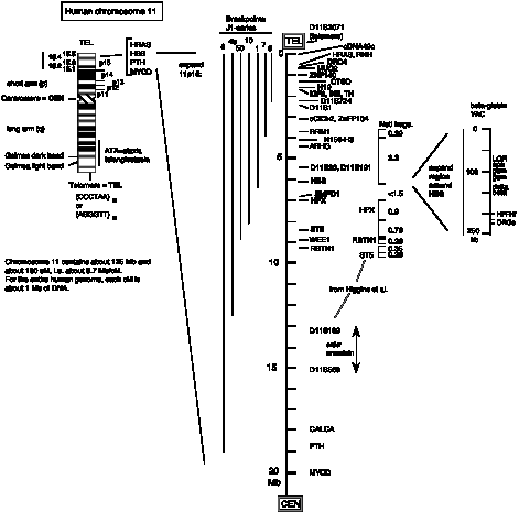
Multiple genes per band on mammalian chromosomes

Fig. 4.27 gives a view of human chromosome 11 at several different levels of resolution. The region 11p15 has many genes of interest, including genes whose products regulate cell growh (HRAS), determination and differentiation of muscle cells (MYOD), carbohydrate metabolism (INS), and mineral metabolism (PTH). The b-globin gene (HBB) and its closely linked relatives are also in this region. A higher resolution view of 11p15, based on a compilation of genetic and physical mapping (Cytogenetics and Cell Genetics, 1995) is shown next to the classic ideogram (banding pattern). This is in a scale of millions of base pairs, and one can start to get a feel for gene density in this region. Interestingly, it varies quite a lot, with the gene-dense sub-bands near the telomeres; these may correspond to the T-bands discussed above. Other genes appear to be more widely separated. For instance, each of the b-like globin genes is separated by about 5 to 8 kb from each other (see the map of the YAC, or yeast artificial chromosome, carrying the b-like globin genes), and this gene cluster is about 1000 kb (i.e. 1 Mb) from the nearest genes on the map. However, further mapping will likely find many other genes in this region. Now even more information is available at the web sites mentioned earlier.

Figure 4.27.

The relationship between recombination distances and physical distances varies substantially among organisms. In human, one centiMorgan (or cM) corresponds to roughly 1 Mb, whereas in yeast 1 cM corresponds to about 2 kb, and this value varies at least 10-fold along the different yeast chromosomes. This is a result of the different frequencies of recombination along the chromosomes.

Specialized regions of chromosomes

Centromere: region responsible for segregation of chromosomes at mitosis and meiosis.

The centromere is a constricted region (usually) toward the center of the chromosome (although it can be located at the end, as with mouse chromosomes.)

It contains a kinetochore, a fibrous region to which microtubules attach as they pull the chromosome to one pole of the dividing cell.

DNA sequences in this region are highly repeated simple sequences (in Drosophila, the unit of the repeat is about 25 bp long, repeated hundreds of times).

Specific proteins are at the centromere, and are now intensely investigated.

Telomere: forms the ends of the linear DNA molecule that makes up the chromosome.

The telomeres are composed of thousands of repeats of CCCTAA in human. Variants of this sequence are found in the telomeres in other species.

Telomeres are formed by telomerase; this enzyme catalyzed the synthesis of more ends at each round of replication to stabilize linear molecules.

The principal proteins in chromatin are histones.

Composition of chromatin

Various biochemical methods are avialable to isolated chromatin from nuclei. Chemical analysis of chromatin reveals proteins and DNA, with the most abundant proteins being the histones. A complex set of less abundant histones are referred to as the nonhistone chromosomal proteins.

The histones and DNA present in equal masses.

Mass Ratio DNA: histones: nonhistone proteins: RNA

= 1: 1: 1: 0.1

Histones are small, basic (positively charged), highly conserved proteins. They bind to each other to form specific complexes, around which DNA wraps to form nucleosomes. The nucleosomes are the fundamental repeating unit of chromatin.

There are 5 histones, 4 in the core of the nucleosome and one outside the core.

H3, H4: Arg rich, most conserved sequence ü

ý CORE Histones

H2A, H2B: Slightly Lys rich, fairly conservedþ

H1: very Lys rich, most variable in sequence between species.

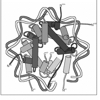
X-ray diffraction studies of histone complexes and the nucleosome core have provided detailed insight into how histones interact with each other and with DNA in this fundamental entity of chromatin structure.

Key reference: "Crystal structure of the nucleosome core particle at 2.8 Å resolution" by Luger, K. Mader, A., Richmond, R.K., Sargent, D.F. & Richmond, T.J. in Nature 389: 251-260 (1997)

Histone interactions via the histone fold.

The core histones have a highly positively charged amino-terminal tail, and most of the rest of the protein forms an a-helical domain. Each core histone has at least 3 a-helices.

Fig. 4.28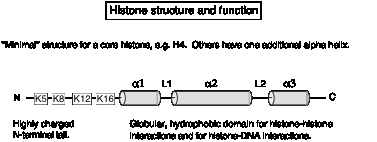

The a-helical domain forms a characteristic histone fold, in which shorter a1 and a3 helices are perpendicular to the longer a2 helix. The a-helices are separated by two loops, L1 and L2. The histone fold is the dimerization domain between pairs of histones, mediating the formation of crescent-shaped heterodimers H3-H4 and H2A-H2B. The histone-fold motifs of the partners in a pair are antiparallel, so that the L1 loop of one is adjacent to the L2 loop of the other.

Fig. 4.29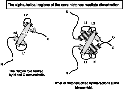

A structure very similar to the histone fold has now been seen in other nuclear proteins, such as some subunits of TFIID, a key component in the general transcription machinery of eukaryotes. It also serves as a dimerization domain for these proteins.

Two H3-H4 heterodimers bind together to form a tetramer.

Nucleosomes are the subunits of the chromatin fiber.

The most extended chromatin fiber is about 10 nm in diameter. It is composed of a series of histone-DNA complexes called nucleosomes.

Principal lines of evidence for this conclusion are:

a. Observations of this 10 nm fiber in the electron microscope showed a series of bodies that looked like beads on a string. We now recognize the beads as the nucleosomal cores and the string as the linker between them.

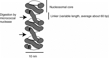
b. Digestion of DNA in chromatin or nuclei with micrococcal nuclease releases a series of products that contain DNA of discrete lengths. When the DNA from the products of micrococcal nuclease digestion was run on an agarose gel, the it was found to be a series of fragments of 200 bp, 400 bp, 600 bp, 800 bp, etc. , i.e. integral multiples of 200 bp. This showed that cleavage by this nuclease, which has very little sequence specificity, was restricted to discrete regions in chromatin. Those regions of cleavage are the linkers.

c. Physical studies, including both both neutron diffraction and electron diffraction data on fibers and most recently X-ray diffraction of crystals, have provided more detailed structural information.

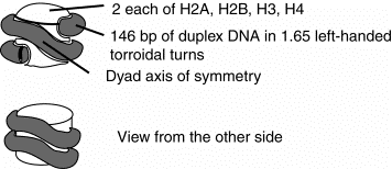
2. The nucleosomal core is composed of an octamer of histones with 146 bp of duplex DNA wrapped around it in 1.65 very tight turns. The octamer of histones is actually a tetramer H32H42 at the central axis, flanked by two H2A-H2B dimers (one at each end of the core.

Figure 4.30. Schematic views of the nucleosomal core:

The 10 nm fiber is composed of a string of nucleosomal cores joined by linker DNA. The length of the linker DNA varies among tissues within an organism and between species, but a common value is about 60 bp. The nucleosome is the core plus the linker, and thus contains about 200 bp of DNA.

Figure 4.31. A string of nucleosomes

Detailed structure of the nucleosomal core.

Path of the DNA and tight packing

The 146 bp of DNA is wrapped around the histone octamer in 1.65 turns of a flat, left-handed torroidal superhelix. Thus 14 turns or "twists" of the DNA are in the 1.65 superhelical turns, presenting 14 major and 14 minor grooves to the histone octamer. Pancreatic DNase I will cleave DNA on the surface of the core about every 10 bp, when each twist of the DNA is exposed on the surface.

The DNA superhelix has an average radius of 41.8 Å and a pitch of 23.9 Å. This is a very tight wrapping of the DNA around the histones in the core - note that the duplex DNA on one turn is only a few Å from the DNA on the next turn! The DNA is not uniformly bent in this superhelix. As the DNA wraps around the histones, the major and then minor grooves are compressed, but not in a uniform manner for all twists of the DNA. G+C rich DNA favors the major groove compression, whereas A+T rich DNA favors the minor groove compression. This is an important feature in translational positioning of nucleosomes and could also affect the affinity of different DNAs for histones in nucleosomes.

The DNA phosphates have high mobility when not contacting histones; the DNA phosphates facing the solvent are much more mobile than is seen with other protein-DNA complexes.

Figure 4.32. A cross-sectional view of the nucleosome core showing histone heterodimers and contacts with DNA. This images corresponds to the proteins and DNA in about one half of the nucleosome.

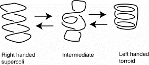
The left-handed torroidal supercoils of DNA in nucleosomal cores is the equivalent of a right-handed, hence negative, supercoil. Thus the DNA in nucleosomes is effectively underwound.

Figure 4.33.

Histones in the nucleosome core particle:

The protein octamer is composed of four dimers (2 H2A-H2B pairs and 2 H3-H4 pairs) that interact through the "histone fold". The two H3-H4 pairs interact through a 4-helix bundle formed between the two H3 proteins to make the H32H42 tetramer. Each H2A-H2B pair interacts with the H32H42 tetramer through a second 4-helix bundle between H2B and H4 histone folds.

The histone-fold regions of the H32H42 tetramer bind to the center of of the DNA covering a total of about 6 twists of the DNA, or 3 twists of DNA per H3-H4 dimer. Those of the H2A-H2B dimers cover a comparable amount of DNA, 3 twists per dimer. Additional helical regions extend from the histone fold regions and are an integral part of the the core protein within the confines of the DNA superhelix.

Histone-DNA interactions in the core particle.

The histone-fold domain of the heterodimers (H3-H4 and H2A-H2B) bind 2.5 turns of DNA double helix, generating a 140˚ bend. The interaction with DNA occurs at two types of sites:

(1) The L1 plus L2 loops at the narrowly tapered ends of each heterodimer form a similar DNA binding site for each histone pair. The L1-L2 loops interact with DNA at each end of the 2.5 turns of DNA.

(2) The a1 helices of each partner in a pair form the convex surface in the center of the DNA binding site. The principal interactions are H-bonds between amino acids and the phosphate backbone of the DNA (there is little sequence specificity to histone-DNA binding). However, there are some exceptions, such a hydrophobic contact between H3Leu65 and the 5-methyl in thymine. An Arg side chain from a histone fold enters the minor groove at 10 of the 14 times it faces the histone octamer. The other 4 occurrences have Arg side chains from tail regions penetrating the minor groove.

Histone tails

The histone N- and C-termial tails make up about 28% of the mass of the core histone proteins, and are seen over about 1/3 of their total length in the electron density map - i.e. that much of their length is relatively immobile in the structure.

The tails of H3 and H2B pass through channels in the DNA superhelix created by 2 juxtaposed minor grooves. One H4 tail segment makes a strong interparticle connection, perhaps relevant to the higher-order structure of nucleosomes.

The most N-terminal regions of the histone tails are not highly ordered in the X-ray crystal structure. These regions extend out from the nucleosome core and hence could be involved in interparticle interactions. The sites for acetylation and de-acetylation of specific lysines are in these segments of the tails that protrude from the core. Post-translational modifications such as acetylation have been implicated in "chromatin remodeling" to allow or aid transcription factor binding. It seems likely that these modifications are affecting interactions between nucleosomal cores, but not changing the structure of the core particle.

Some excellent resources are available on the World Wide Web for visualizing and further investigating chromatin structure and its involvment in nuclear processes.

Dmitry Pruss maintains a site with many good images, including dynamic, step-by-step view of the nuclesomal core beginning with the histone fold domains and ending with a complete core, with DNA.

http://www.average.org/~pruss/nucleosome.html

Another good site is from J.R. Bone:

http://rampages.onramp.net/~jrbone/chrom.html

Higher order chromatin structure

1. The 10 nm fiber composed of nucleosomal cores and spacers is folded into higher order structures for much of the DNA in chromatin. In fact, the 10 nm fiber with the beads-on-a-string appearance in the electron microscope was prepared at very low salt concentrations and is free of histone H1.

2. In the presence of H1 and at more physiological salt concentrations, chromatin forms a 30 nm fiber. The exact structure of this fiber remains a point of considerable debate, and one cannot rule the possibility of multiple structure in this fiber.

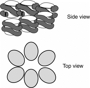
3. One reaonable model is that the 10 nm fiber coils around itself to generate a solenoid that is 30 nm in diameter, with 6 nucleosomes per turn of of the solenoid.

Histone H1 binds to the outer surface of the nucleosomal core, interacting at the points of DNA entry and exit. H1 molecules can be cross-linked to each other with chemical reagents, indicating that the H1 proteins also interact with each other. Interactions between H1 proteins, each bound to a nucleosomal core, may be one of the forces driving the formation of the 30 nm fiber.

Figure 4.34. Model for one turn of the solenoid in the 30 nm fiber.

4. Each level of chromatin structure produces a more compact arrangment of the DNA. This can be described in terms of a packing ratio, which is the length of the DNA in an extended state divided by the length of the DNA in the more compact state.

For the 10 nm fiber, the packing ratio is about 7, i.e. there are 7mm of DNA per mm of chromatin fiber. The packing ratio in the core is higher (see problems), but this does not include the additional, less compacted DNA in the spacer. In the 30 nm fiber, the packing ratio is about 40, i.e. there 40mm DNA per mm of chromatin fiber.

5. The 30 nm fiber is probably the basic constituent of both interphase chromatin and mitotic chromosomes. It can be compacted further by additional coils and loops. One of the key issues in gene regulation is the nature of the chromating fiber in transcriptionally acative euchromatin. Is it the 10 nm fiber? the 30 nm fiber? some modification of the latter? or even some higher order structure? These are topics for current research.

Additional Readings

Britten RJ, Kohne DE. (1968) Repeated sequences in DNA. Hundreds of thousands of copies of DNA sequences have been incorporated into the genomes of higher organisms. Science 161:529-540

Wetmur and Davidson (1968)The rate constant for renaturation is inversely proportional to sequence complexity. J. Molecular Biology 34:349-370.

Davidson EH, Hough BR, Amenson CS, Britten RJ. (1973) General interspersion of repetitive with non-repetitive sequence elements in the DNA of Xenopus. J. Molecular Biology 77:1-23.

Fleischmann RD, Adams MD, White O, Clayton RA, Kirkness EF, Kerlavage AR, Bult CJ, Tomb JF, Dougherty BA, Merrick JM, et al. (1995) Whole-genome random sequencing and assembly of Haemophilus influenzae Rd. Science. 269:496-512

Adams MD, Celniker SE, Holt RA, Evans CA, Gocayne JD, Amanatides PG, Scherer SE,

Li PW, Hoskins RA, Galle RF, George RA, Lewis SE, Richards S, Ashburner M,

Henderson SN, Sutton GG, Wortman JR, Yandell MD, Zhang Q, Chen LX, Brandon RC,

Rogers YH, Blazej RG, Champe M, Pfeiffer BD, Wan KH, Doyle C, Baxter EG, Helt G,

Nelson CR, Gabor GL, Abril JF, Agbayani A, An HJ, Andrews-Pfannkoch C, Baldwin

D, Ballew RM, Basu A, Baxendale J, Bayraktaroglu L, Beasley EM, Beeson KY, Benos

PV, Berman BP, Bhandari D, Bolshakov S, Borkova D, Botchan MR, Bouck J,

Brokstein P, Brottier P, Burtis KC, Busam DA, Butler H, Cadieu E, Center A,

Chandra I, Cherry JM, Cawley S, Dahlke C, Davenport LB, Davies P, de Pablos B,

Delcher A, Deng Z, Mays AD, Dew I, Dietz SM, Dodson K, Doup LE, Downes M,

Dugan-Rocha S, Dunkov BC, Dunn P, Durbin KJ, Evangelista CC, Ferraz C, Ferriera

S, Fleischmann W, Fosler C, Gabrielian AE, Garg NS, Gelbart WM, Glasser K,

Glodek A, Gong F, Gorrell JH, Gu Z, Guan P, Harris M, Harris NL, Harvey D,

Heiman TJ, Hernandez JR, Houck J, Hostin D, Houston KA, Howland TJ, Wei MH,

Ibegwam C, Jalali M, Kalush F, Karpen GH, Ke Z, Kennison JA, Ketchum KA, Kimmel

BE, Kodira CD, Kraft C, Kravitz S, Kulp D, Lai Z, Lasko P, Lei Y, Levitsky AA,

Li J, Li Z, Liang Y, Lin X, Liu X, Mattei B, McIntosh TC, McLeod MP, McPherson

D, Merkulov G, Milshina NV, Mobarry C, Morris J, Moshrefi A, Mount SM, Moy M,

Murphy B, Murphy L, Muzny DM, Nelson DL, Nelson DR, Nelson KA, Nixon K, Nusskern

DR, Pacleb JM, Palazzolo M, Pittman GS, Pan S, Pollard J, Puri V, Reese MG,

Reinert K, Remington K, Saunders RD, Scheeler F, Shen H, Shue BC, Siden-Kiamos

I, Simpson M, Skupski MP, Smith T, Spier E, Spradling AC, Stapleton M, Strong R,

Sun E, Svirskas R, Tector C, Turner R, Venter E, Wang AH, Wang X, Wang ZY,

Wassarman DA, Weinstock GM, Weissenbach J, Williams SM, WoodageT, Worley KC, Wu

D, Yang S, Yao QA, Ye J, Yeh RF, Zaveri JS, Zhan M, Zhang G, Zhao Q, Zheng L,

Zheng XH, Zhong FN, Zhong W, Zhou X, Zhu S, Zhu X, Smith HO, Gibbs RA, Myers EW,

Rubin GM, Venter JC. (2000) The genome sequence of Drosophila melanogaster. Science 287:2185-2195

International Human Genome Sequencing Consortium, I. H. G. S. (2001). Initial sequencing and analysis of the human genome. Nature 409: 860-921.

Rubin, G. M., Yandell, M. D., Wortman, J. R., Gabor Miklos, G. L., Nelson, C. R., Hariharan, I. K., Fortini, M. E., Li, P. W., Apweiler, R., Fleischmann, W., Cherry, J. M., Henikoff, S., Skupski, M. P., Misra, S., Ashburner, M., Birney, E., Boguski, M. S., Brody, T., Brokstein, P., Celniker, S. E., Chervitz, S. A., Coates, D., Cravchik, A., Gabrielian, A., Galle, R. F., Gelbart, W. M., George, R. A., Goldstein, L. S., Gong, F., Guan, P., Harris, N. L., Hay, B. A., Hoskins, R. A., Li, J., Li, Z., Hynes, R. O., Jones, S. J., Kuehl, P. M., Lemaitre, B., Littleton, J. T., Morrison, D. K., Mungall, C., O'Farrell, P. H., Pickeral, O. K., Shue, C., Vosshall, L. B., Zhang, J., Zhao, Q., Zheng, X. H., Zhong, F., Zhong, W., Gibbs, R., Venter, J. C., Adams, M. D. and Lewis, S. (2000). Comparative genomics of the eukaryotes. Science 287: 2204-15.

Venter, J. C., Adams, M. D., Myers, E. W., Li, P. W., Mural, R. J., Sutton, G. G., Smith, H. O., Yandell, M., Evans, C. A., Holt, R. A., Gocayne, J. D., Amanatides, P., Ballew, R. M., Huson, D. H., Wortman, J. R., Zhang, Q., Kodira, C. D., Zheng, X. H., Chen, L., Skupski, M., Subramanian, G., Thomas, P. D., Zhang, J., Gabor Miklos, G. L., Nelson, C., Broder, S., Clark, A. G., Nadeau, J., McKusick, V. A., Zinder, N., Levine, A. J., Roberts, R. J., Simon, M., Slayman, C., Hunkapiller, M., Bolanos, R., Delcher, A., Dew, I., Fasulo, D., Flanigan, M., Florea, L., Halpern, A., Hannenhalli, S., Kravitz, S., Levy, S., Mobarry, C., Reinert, K., Remington, K., Abu-Threideh, J., Beasley, E., Biddick, K., Bonazzi, V., Brandon, R., Cargill, M., Chandramouliswaran, I., Charlab, R., Chaturvedi, K., Deng, Z., Di Francesco, V., Dunn, P., Eilbeck, K., Evangelista, C., Gabrielian, A. E., Gan, W., Ge, W., Gong, F., Gu, Z., Guan, P., Heiman, T. J., Higgins, M. E., Ji, R. R., Ke, Z., Ketchum, K. A., Lai, Z., Lei, Y., Li, Z., Li, J., Liang, Y., Lin, X., Lu, F., Merkulov, G. V., Milshina, N., Moore, H. M., Naik, A. K., Narayan, V. A., Neelam, B., Nusskern, D., Rusch, D. B., Salzberg, S., Shao, W., Shue, B., Sun, J., Wang, Z., Wang, A., Wang, X., Wang, J., Wei, M., Wides, R., Xiao, C., Yan, C. (2001). The sequence of the human genome. Science 291: 1304-1351.

The Arabidopsis Genome Initiative (2000) Sequence of the Arabidopsis thaliana genome. Nature 408:796-815.

QUESTIONS

CHAPTER 4

GENOMES AND CHROMOSOMES

4.3 (BPA) Answer the following questions with reference to the figure below.

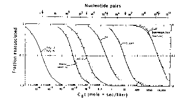
Figure for 4.3 Reassociation of nucleic acids, sheared to 500-nucleotide fragments, from various sources [Derived fom R. J. Britten and D. Kohne, Science, 161,529 (1968).]

a) How many of these DNA preparations contain more than one frequency class of sequences? Explain your answer.

b) If the genome size of E. coli is taken to be 4.5 x 106 nucleotide pairs, what is the genome size of T4?

c) What is the complexity of mouse satellite DNA?

d) Mouse satellite DNA represents 10% of the mouse genome. What is the repetition number for mouse satellite sequences, given that the haploid genome size is 3.2 x 109 nucleotide pairs?

e) The calf genome is the same size as the mouse genome. What fraction of the calf genome is composed of unique sequences?

4.4 Let’s imagine that you obtained a DNA sample from an armadillo and measured the kinetics of renaturation of the genomic DNA. A standard of bacterial DNA (N = 3 x 106 bp) was also renatured under identical conditions. Three kinetic components were seen in the armadillo DNA C0t curve, renaturing fast, medium or slow. The fraction of the genome occupied by each component (f) and the C0t value for half-renaturation (Cot 1/2(measured)) are as follows:

Component f Cot 1/2(measured)

fast 0.2 10-4

medium 0.4 10-1

slow 0.4 104

a) Use the information provided to calculate the Cot 1/2(pure), the complexity (N), and the repetition frequency (R) for each component. Assume that the slowly renaturing component is single copy.

b) Calculate the genome size (G) of the armadillo under the assumption that the slowly renaturing component is single copy.

c) Which of the following sequences could be a member of the fast renaturing component?

GACTCAGACTCAGACTCA

ATATATATATATATATAT

ACTGCCACGGGATACTGC

GCGCGC

4.5 RNA abundance

The availability of cloned DNA probes for many genes has greatly facilitated the analysis of amounts of RNAs in different cells or under different conditions. For instance, it is very common to label a DNA probe that will hybridize to mRNA; the DNA comes from either a cDNA clone or a genomic clone containing an exon. The labeled probe is then hybridized to total or polyA-containing RNA (the latter is called polyA+ RNA, and is roughly equivalent to mRNA) from a cell. The concentration of the probe is much greater than the concentration of the target mRNA for the specific gene, thus the probe is in vast excess and all mRNA from the gene of interest should be driven into a duplex with the probe. The amount of probe protected from digestion by a single-strand specific nuclease such as nuclease S1 gives a measure of the amount of the specific mRNA that is in the cell. (This situation differs in some important aspects from the materialon estimating numbers of genes expressed and abundance from the kinetics of RNA-driven reactions. In that material, one was looking at entire populations of mRNAs, whereas in this situation, one is looking at only one mRNA - the one complementary to the labeled probe.)

[Two technical notes: The diagnostic assay here measures the amount of labeled DNA in duplex and the unhybridized DNA is digested. If the DNA probe is originally double-stranded, it is initially denatured prior to hybridization, but now how do you distinguish between nuclease protection arising from DNA-mRNA duplexes versus those that arise from the two strands of DNA reannealing? The cleanest approach is to just synthesize and label the strand of DNA complementary to the mRNA; this can be done by appropriate choices of primers for synthesis of DNA from plasmids carrying the DNA used as a probe. Alternatively, a labeled duplex DNA probe can be prepared that extends past the mRNA coding portion of a gene, so that the DNA-DNA duplex resulting from reannealing is larger than the DNA-RNA duplex resulting from hybridization to mRNA. Also, hybridization conditions with high concentrations of salt and formamide are used that favor DNA-RNA duplexes over DNA-DNA duplexes. (2) An equivalent approach is to synthesize an RNA probe derived from the cloned DNA; this "complementary RNA" forms a stronger duplex with the mRNA than does cDNA; RNA-RNA duplexes are stronger than RNA-DNA duplexes under conditions of high salt and formamide concentrations. The fragments protected from digestion by RNases are then detected.]

a) Murine erythroleukemia (MEL) cells are equivalent to proerythroblasts, immortalized by the Friend virus complex so that they can grow continuously in culture. Treatment with small organic compounds like dimethylsulfoxide (DMSO) will induce them to mature on to erythroblasts, with a substantial increase in the expression of erythroid specific genes (the mechanism for this induction is still unknown). Let's say that you isolated total RNA from both uninduced (untreated) cells and an equal number of DMSO-induced cells. The RNA samples were hybridized to an excess of a radiolabeled DNA probe from a mouse b-globin gene, and the amount of probe hybridized to the mRNA was determined by treatment of the samples with nuclease S1, electrophoresis on a denaturing polyacrylamide gel, and measuring the amount of radioactivity in the fragment resulting from the mRNA-DNA duplex. An illustration of the heteroduplex, the nuclease S1 treatment, and the resultant autoradiograph of the gel are shown below. The protected fragment from uninduced cells had 10,000 cpm, and the protected fragment from induced cells had 500,000 cpm. A negative control with RNA from a T-lymphocytic cell line, which produces no globin mRNA, gave no protection, i.e. 0 cpm for the diagnostic fragment. The expression of this b-globin gene is induced how much in MEL cells treated with DMSO?

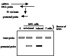
b) The previous assay gives the relative amounts of the mRNA under the two conditions, and this is an extremely powerful and widely used assay. But what does this mean in terms of mRNA molecules per cell, i.e. how does the abundance change upon induction? One can alter this assay somewhat to get a measure of abundance, similar in principle to the calculations in Section VIIF. First, one needs a measure of the number of mRNA molecules per cell. Let's say that you harvested 107 MEL cells and isolated 3 mg of polyA+ RNA (essentially mRNA). What is the total number of mRNA molecules per MEL cell, assuming an average length of mRNA of 2000 nucleotides?

c) If one labels the RNA in the MEL cells, e.g. by growing the cells in the presence of [3H] uridine, which is incorporated only into RNA, then the isolated, labeled polyA+ RNA can be hybridized to an excess of the (now unlabeled) DNA complementary to the mRNA of interest. RNA in duplex with DNA can be detected by its protection from digestion by nucleases such as RNase A and RNase T1; the resulting autoradiograph would look something like that shown below, with bands containing more radioactivity represented as a darker fill. Since the DNA is still in excess, all the mRNA complementary to the probe should be driven into duplex, and one can readily measure the fraction of polyA+ RNA complementary to each probe. The following table provides some representative, idealized data for polyA+ RNA from uninduced and induced MEL cells, including the total input RNA (not treated with nucleases) and the amount protected from nuclease digestion by hybridization with an excess of b-globin gene DNA, DNA encoding the erythroid transcription factor GATA1, and DNA encoding ovalbumin (which is not expressed in MEL cells, i.e. it is a negative control). What fraction of the mRNA (or polyA+ RNA) is composed of mRNA from these three genes, and what is their abundance in uninduced and induced cells?

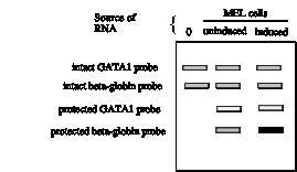
DNA probe	cpm protected uninduced MEL cells	cpm protected induced MEL cells
[input labeled RNA]	[1,000,000]	[1,000,000]
b-globin	5,000	250,000
GATA1	25	25
ovalbumin	0	0

d) In general, what is the distribution of mRNAs in a particular type of differentiated cell, i.e. how abundant are the different complexity classes of mRNA?

Use of databases of sequences, mutations, and functional data

4.6 We used arginine biosynthesis to illustrate complementation analysis and construction of a pathway. The steps involved in arginine synthesis are also part of the urea cycle. One of the enzymes catalyzes the formation of citrulline from carbamoyl phosphate and ornithine. Let's find out more about this enzyme, called ornithine transcarbamoylase, or OTC.

Use your favorite Web browser to go to the URL for NCBI (National Center for Biotechnology Information).

http://www.ncbi.nlm.nih.gov/

Click on the Entrez button. Entrez provides a portal to many types of information at this server. Let's start with DNA and protein sequences.

Click on the Nucleotides button.

Enter "X00210" and press the Search button. Do not enter the quotation marks, and those are zeros and a one, not O or l.

You should get a report on the gene for OTC in E. coli, called argI.

a) How large is the protein-coding region, from translation initiation codon to the termination codon? How big is the encoded protein?

b) Where is the argI gene on the E. coli chromosome? Go back to the Entrez server (where you clicked on Nucleotides before). Click on Genomes, and then select Escherichia coli. Enter "argI" in the Search window (don't enter the quotes, and that is the letter I "eye" not a "one").

4.7 Is the E. coli OTC protein related to any other proteins in the sequence databases? You need to get the protein sequence, which you can do by clicking on argI while you are at the genome map, or you can go back to the entry for the gene (accession number X00210). If you are at the GenBank Report for entry X00210, you need to click on the Protein button at the top of the page, and then select FastA Report from the next page. (If you take the default path the GenPept Report, that is OK, you can get the FastA Report from there as well.) Make a copy of this OTC sequence in FastA format (you may want to save it in another program, e.g. your favorite word processor, for convenience).

Now click on the Blast button at the top of the page, and at the next page select Basic Blast search. At the Blast server, select blastp from the pull-down menu next to Program (this aligns protein sequences; the default blastn aligns nucleotide sequences), and paste the E. coli OTCsequence in FastA format into the input window. Note that the pull-down menu gives you the option of entering the accession number (40962) instead of the sequence. The default sequence databases are nr, the non-redundant compilation of databases from the US, Europe and Japan. We'll use that, but note that a pull-down menu allows you to select other databases.

a) Click on the Submit Query button. When the job finally runs (this can take a minute or more when the Server is busy) what do you see?

b) Is the E. coli OTC protein related to any human protein? Scroll down the table of hits, past many bacterial OTCs (Neisseria, Pyrococcus ...) until you run into some mammalian hits. With a score of 172, you should find a hyperlink to sp|P00480|OTC_HUMAN ORNITHINE CARBAMOYLTRANSFERASE PRECURSOR. Click on this hyperlink.

4.8 The entry for human OTC (P00480, which is the same as 400687) is quite long.

a) What occupies much of the feature table? What does this tell you about the OTC gene in humans?

b) Using either the features table for the GenBank entry 400687 (or P00480) or better yet, go back to the home page for NCBI and click on the OMIM button to go to the On-Line Medelian Inheritance In Man (from Victor McKusick, M.D.). Where is the gene? What happens in OTC deficiency?

4.9 What do the aligned amino acid sequences of the bacterial and human proteins tell you? Do conserved regions correlate with functional regions? For instance, does mutation of any amino acids in the conserved regions lead to a phenotype in humans?

Since the Blast search generated so many hits with higher scores than the E. coli- human pair, we will have to use a different tool to see the alignment. At the Blast server top page (where you selected Basic Blast search before), select Blast 2 sequences. This utility allows you to enter any two sequences and generate a pairwise alignment by the program Blast2. You should use the human and E. coli OTC protein sequences or their accession numbers, and be sure to choose blastp as the program. When doing this in July of 1998, I ran into a problem with the utility making a duplicate of each sequence I entered (I don't know if that was a problem at my end or theirs); this is likely a temporary condition. If you encounter a problem, try a different Server, such as the Sequence Analysis Server at http://genome.cs.mtu.edu/sas.html. Choose Pairwise Sequence Alignment, enter your sequences and run GAP or SIM on protein sequences.

Chromatin

4.10 One of the important early pieces of evidence that helped define the structure of the nucleosome was the pattern of nuclease cleavage in chromatin. In this experiment, chromatin was treated briefly with an enzyme, micrococcal nuclease, that degrades DNA, then all protein was removed and the and the purified DNA resolved by electrophoresis. A regular pattern of broad bands was seen; the average sizes of the DNA fragments were multiples of 200 bp, i.e. 200, 400, 600, 800 bp, etc. What does this result tell you about chromatin structure? The bands of DNA bands were thick and spread out rather than sharp; what does this tell you about the positions of cleavage by micrococcal nuclease?

4.11 Which histones are in the core of the nucleosome? What are the protein-protein interactions in the core? What protein domains mediate these interactions?

4.12 The mammalian virus SV40 has minichromosomes in which the circular duplex DNA is packaged into nucleosomes. When histones are removed from the minichromosomes, the resulting DNA is found to be negatively supercoiled. What does this tell you about the state of the DNA in the minichrosomes and the path of the DNA around the nucleosome?

4.13 Are the following statements true or false?

a) The DNA coils around the histones about 1.65 turns per nucleosomal core.

b) The DNA in chromatin containing actively transcribed genes is usually more sensitive to DNases than is the DNA in nontranscribed chromatin.

4.14 The packing ratio of a nucleic acid-protein complex is the ratio between the length of the naked DNA in normal B form to the length of the protein-DNA structure. For instance, if a set of proteins folded a DNA molecule of 100 Å into a structure that is 25 Å long, this structure has a packing ratio of 4.

a) Given the dimensions of the nucleosome structure, what is the packing ratio for the DNA in the nucleosome core? Note that the pitch is the distance between the midpoints of the DNA duplex as it turns around the histones in the core.

b) If the nucleosomes are tight-packed into a solenoid with 6 nucleosomes per turn, what is the packing ratio now? Assume that each turn of the solenoid translates 110 Å, i.e. the distance between the midpoints of nucleosomes in successive turns of the solenoid is 110 Å.

4.15 How close are the edges of the DNA as it curves around the surface of the nucleosomal core?